
The Atomic Nucleus
E N D
Presentation Transcript
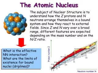
The Atomic Nucleus The subject of Nuclear Structure is to understand how the Z protons and N neutrons arrange themselves in a bound system and how they react to external fields. Since Z and N vary over a broad range, different features are expected depending on the mass number and on the N/Z ratio. What is the effective NN interaction?What are the limits of existence for bound nuclei (driplines)?
The Shell Model There is a “surprising” analogy between the description of bound electrons in atoms and bound nucleons in atomic nuclei. Nuclear Shell Model (M.Mayer et al, 1948-49) This model is a highly successful one, but the prediction capabilities are somewhat limited when going to nuclei far from stability Need to “tune” the model parameters collecting information on such nuclei!
Shell structure Cooper pairing Collective modes Nuclear excitations
X-ray burst 4U1728-34 331 Frequency (Hz) 330 329 328 327 10 15 20 Time (s) Nuclear Physics and Stellar Nucleosynthesis • What is the origin of elements heavier than Iron? • How do stars burn and explode? • What is the structure of a neutron star? p process s-process r process rp process Nova Neutron star Crust processes T Pyxidis stellar burning protons neutrons
neutron drip-line Stablenuclei heavy-ion collisions 10 ρ0 proton drip-line Nuclei and Stars supernovae
Symmetry Energy: Nuclei and Stars The symmetry energy determines the dynamics of supernovae explosions and the pressure in neutron stars: Psym(ρ,δ) = ρ2 (∂Esym/∂ ρ ) δ2 = ρ0 Esym (ρo) u +1 δ2 Esym (ρ) = Esym (ρo) u u= ρ/ρo Observables (input to the models): Dynamics of heavy-ion collisions at different N/Z ratios Structure of nuclei far from stability: single-particle and collective properties
How can we perform nuclear structure studies? • In order to study the structure of nuclei, we need to find them in an excited state and to observe the radiation (light particles, electrons, g-rays) which they do emit during the de-excitation. • Excited nuclei can be populated “naturally” by decay of long-lived radioactive nuclei, or by reactions induced by cosmic rays • Excited nuclei can be populated “artificially” by inducing nuclear reactions in our laboratories, using accelerators
TANDEM PIAVE ALPI COMPLEX SC BoosterALPI 68 SC Quarter Wave Resonators (Nb, Nb/Cu) Veq ~ 48 MV, species from 28Si to 197Au Injected by Tandem or PIAVE PI Injector PIAVE VT ~ 14,5 MV From H to 197Au, E = 30 ÷ 1.5 MeV/A CW or pulsed ECR on 350 kV platform SC-RFQs and QWRs Veq ~ 8 MV Fully operational with noble Gases; ECRIS replacement in Spring 2008 XTU-Tandem
Producing nuclei far from stability Using stable beams at energies close to the Coulomb barrier, with a careful choice of the reaction mechanism it is possible to populate nuclei far from stability in different regions of the chart of nuclides
Observing nuclei far from stability • Following the production of excited, exotic nuclei, there are two basic alternatives, implying quite different experimental problems: • Transport the excited nuclei elsewhere and observe the (delayed) decays (or chains of decays) off-line • Observe the prompt decays on-line, as they are produced
Gamma Spectroscopy • The observation of the electromagnetic radiation (photons or g-rays) emitted by the excited nuclei provides one of the most sensitive tools to investigate the nuclear structure • The emission of g-rays is a well understood process from the theoretical point of view, hence the smallest effects can provide valuable information on the nuclear structure • Contrary to the detection of particles, high resolution is possible
Detectors • A detector is an object translating the arrival of a radiation quantum into a (measurable) electric signal which can be: • generated outside of the active volume of the detector (eg scintillators coupled to photomultiplier tubes) • generated inside of the active volume of the detector (eg semiconductor detectors)
Detector I Current mode A possible mode of operation consists in measuring the average current produced within the detector. This mode of operation is not much used in spectroscopy since there is no information on the energy of the individual radiation quanta, only on their rate.
Pulse mode Here the information on energy and time of arrival of the individual quanta is preserved. Typically, the charge flowing at the detector electrodes is collected by a preamplifier, which we can approximate by a RC circuit. RC small compared to the charge collection time: the output signal is basically the same as the current signal: V(t)=R i(t) RC large compared to the charge collection time: the output signal rises as the current signal and decays exponentially with time constant RC. Its amplitude V=Q/C is proportional to the energy if C is constant.
Spectra The usual way to visualize the response of a detector is a differential spectrum, namely a histogram in which each channel content is the number of events with amplitude within the “bin”. The integral version is not as widely used. Integral Differential
Resolution When monochromatic radiation hits a detector, one expects that the response of the detector is always the same, in other words, that a peak appears in the differential spectrum. The resolutionR is defined as the ratio between the peak full width at half maximum (FWHM) and its position, R=FWHM/H0, but conventionally the values of FWHM and energy can be provided. For gaussian peaks, the statistical limit is: where N is the peak area. In practice the resolution can be better than such a limit and the Fano factor F<1 is introduced:
Efficiency • The absolute efficiency is defined as the ratio between the number of detected and emitted quanta • The intrinsic efficiency is defined as the ratio between the number of detected quanta and the number of quanta hitting the detector • These two quantities are related by geometrical factors • The peak efficiencies (absolute and intrinsic) are defined in a similar way
Interaction of radiation with matter • As a rule of thumb: • Charged particles (electrons, protons) release their energy in a gradual and continuous way • Neutral particles (neutrons, photons) release their energy through “catastrophic events” changing their energy and/or nature in a radical way
Photon Interaction Mechanisms ~ 100 keV ~1 MeV ~ 10 MeV g-ray energy Photoelectric Compton Scattering Pair Production
Photoelectric Absorption A photon can interact with an atom,releasing an electron with energy:Ee=Eg-Ebwhere Eb is the electron binding energy. The ionised atom can then rearrange its electrons, emitting X-rays which are typically reabsorbed. In first approximation, the cross section for photoelectric absorption is: Shell effects, however, are typically quite evident.
Compton Scattering Compton scattering is the elastic scattering of a photon on an electron. For a free electron, the energy of the scattered photon depends on the scattering angle q: The energy of the scattered electron in the extreme cases, q=0, q=p is: From which we obtain the gap between the photon energy and the maximum electron energy (which for large values of Eg is approximately 256 keV):
Compton Scattering The angular distribution of the scattered photon is described by the Klein-Nishina formula: where a=Eg/mec2 and re is the classical electron radius.For photon energies larger than a few hundred keVs the angular distribution is highly anisotropical and peaked to small forward angles. It strongly decreases with the increasing photon energy.
Continuum Compton The spectrum of the scattered electrons can be deduced from the Klein-Nishina formula: where: Since the actual energy deposition is performed by the electrons, photons interacting via Compton scattering will produce a continuum spectrum as shown here. Corrections are needed since electrons are not free, rather bound in materials, producing a smoothening of the actual spectrum (Compton profile) Compton edge 1332 keV photons
Pair production Photons with energy larger than 2mec2can materialize (in the Coulomb field of a nucleus) in an electron-positron pair with total kinetic energy Eg-2mec2.Electron and positron subsequently release their energy in the medium; the positron eventually annihilates releasing two 511 keV photons. • The threshold for this process is 1.022 MeV • This process dominates at high photon energies (Eg> 10 MeV) • This process depends approximately on the square of the atomic number of the medium.
Cross Sections in NaI(Tl) NaI(Tl) Atomic shell K Cross Section Pairprod. Comptonscatt. Photoelectricabs. Energy (MeV)
Cross Sections in Germanium Photoelectric Compton scatt. Pairprod. Mean free path: l(E) = MA/(NAV.r) . 1/SsE l(10 keV) ~ 55 mm l(100 keV) ~ 0.3 cm l(200 keV) ~ 1.1 cm l(500 keV) ~ 2.3 cm l(1 MeV) ~ 3.3 cm
Response function • The response function is the differential spectrum obtained with a detector when hit by monochromatic radiation • We can consider some schematic cases: • Large detectors • Small detectors • Intermediate size detectors
“Large” detectors In the ideal case of a very large detector (with respect to the mean free path of the radiation), the incoming radiation is fully absorbed.Since it is not possible to discriminate the time at which the individual interaction points are produced, the detector is only sensitive to the total energy deposition.
“Large” detectors Ideal Ge sphere, 1 m diametre.3 MeV photons The response function of a “large” detector is very simple and it includes only a full-energy peak (which in most practical cases can be treated as a photopeak). Full-energy peak Lucrecia TAS at GSI Some devices (Total Absorption Spectrometers) are a good implementation of this limit!
“Small” detectors E=1.33MeV In this case there is a high probability that the incoming photons are only partially absorbed.In the response function, besides the full-energy peak, one can identify a continuum generated by photons which underwent Compton scattering and, if the photon energy is larger than 1.022 MeV, peaks due to the missed detection of one or both the annihilation photons (single and double escape peaks). Compton continuum full-energy peak E=3MeV Double escape peak
Full-energy peak Compton continuum Single-escape peak Double-escape peak Intermediate size detectors The situation is qualitatively similar to the case of “small” detectors, although in practice also other components can be identified, due for instance to the environmental background (eg 40K), to the bremsstrahlung radiation, to the X-rays characteristic of the material surrounding the detector and a peak of approximately 250 keV due to the back scattering of the incoming photons. HPGe detector used with the GASP array
152Dy In-beam g-ray spectroscopy What we want … What we get … Problems: complex spectra!Many lines lie close in energy and the “interesting” channels are typically the weak ones ... Our goal is to extract new valuable information on the nuclear structure through the g-rays emitted following nuclear reactions
The nucleus is always full of surprises Instrumentation advances New Science
New tools for new phenomena From Sodium Iodide to Germanium detectors With high-resolution devices the nuclear world seems quite different! Continuous effort to consistently improve our detectors and their response function 104Ag and 106 Ag
Spectroscopic history of 156Dy 156Dy The “spectroscopic history” of 156Dy is a notable example of how the progress with the acceleration and detection techniques leads to better insight on the nuclear structure.
Shape coexistence Transfermium nuclei 100Sn 48Ni 132+xSn 78Ni Challenges in Nuclear Structure • Shell structure in nuclei • Structure of doubly magic nuclei • Changes in the (effective) interactions • Proton drip line and N=Z nuclei • Spectroscopy beyond the drip line • Proton-neutron pairing • Isospin symmetry • Nuclear shapes • Exotic shapes and isomers • Coexistence and transitions • Neutron rich heavy nuclei (N/Z → 2) • Large neutron skins (rn-rp→ 1fm) • New coherent excitation modes • Shell quenching • Nuclei at the neutron drip line (Z→25) • Very large proton-neutron asymmetries • Resonant excitation modes • Neutron Decay
Neutron-rich beams Physics with radioactive beams
Excitation energy Eexc Coupling with continuum Binding energy Angular momentum J Isospin Angular momentum (Deformation) N- Z N+Z Neutron-proton ratio Nuclei under extreme conditions
Nuclei under extreme conditions With state-of-the-art experiments we try to study nuclei under “extreme” conditions in order to collect valuable information to refine the theoretical description and our knowledge of the nuclear interaction Isospin: N/Z ratios much larger (or smaller) than the stability line Spin: highly rotating nuclei Temperature: “hot” nuclei The quest for the spin frontier was a major driving force in the development of modern instrumentation
Producing fast rotating nuclei Following the development of accelerators for heavy ions, it became possible to populate nuclei at high spin The stability of a nucleus under rotation can be estimated using the liquid-drop model. At low frequencies the shape of a rotating drop is oblate, at higher frequency it becomes prolate (Jacobi transition)
Quantum rotors Only a non-spherical quantum object can rotate (around an axis different than the symmetry axis) Here J is the moment of inertia. In case of axially symmetric rotors I can only assume even values because of the symmetry for reflection. Regularly spaced transitions!
Moments of inertia Defining the rotation frequency as: There are two possible expressions for the moment of inertia: Kinematical: requires knowledge of spin Dynamical: requires knowledge of spin differences
Moments of inertia The two definitions of moment of inertia coincide only for rigid rotors (energy strictly proportional to I2) Can we really consider the nucleus a good rigid rotor?
Alignments Rather than rotating the nucleus as a whole, another possibility to generate angular momentum is to align the orbital angular momenta of individual nucleons in high-l orbitals (rotation around a symmetry axis) This process can continue up to the full alignment of all nucleons, producing a band terminating state
Backbending When the rotational frequency is high enough, a pair of nucleons can break (align) with a sudden change in the moment of intertia. The regular sequence of transitions is interrupted. This is known as backbending from the characteristic behaviour of the moment of inertia vs rotational frequency plot.
Deformation How deformed can a nucleus be? Increasing the deformation costs energy and eventually the Coulomb repulsion will cause the nucleus to fission. In particular cases, due to shell effects, a second minimum at large deformation develops, in which (weak) rotational structures can be built How can we enhance these structures experimentally?
Ridges Using at least two detectors in coincidence, weak rotational structures can be enhanced by looking “sideways” at the coincidence matrix, which should result in a “ridge” structure.
Superdeformed bands With the appropriate tools, it was possible to observe discrete transitions from long (20 transitions or more) and weak (populated with a cross section lower than 10-4 of the total cross section) rotational structures. These bands were called superdeformed because the deformation corresponded to extremely elongated shapes (2:1 ratio in the ellipsoid axes)
Linking transitions In most cases, the SD bandhead is “floating” and only J(2) can be determined. Only in a few cases the linking transition(s) between normal deformed and superdeformed states could be observed. These cases are obviously very important since a direct comparison between theory and experiment is possible.