Probabilistic Reasoning over Time
Russell and Norvig, AIMA : Chapter 15 Part A: 15.1 , 15.2. Probabilistic Reasoning over Time. Presented to: Prof. Dr. S. M. Aqil Burney. Presented by: Zain Abbas (MSCS-UBIT). Agenda. Temporal probabilistic agents Inference : Filtering, prediction, smoothing and most likely explanation

Probabilistic Reasoning over Time
E N D
Presentation Transcript
Russell and Norvig, AIMA : Chapter 15 Part A: 15.1 , 15.2 Probabilistic Reasoning over Time Presented to: Prof. Dr. S. M. Aqil Burney Presented by: ZainAbbas (MSCS-UBIT)
Agenda • Temporal probabilistic agents • Inference: Filtering, prediction, smoothing and most likely explanation • Hidden Markov models • Kalman filters
Agenda • Temporal probabilistic agents • Inference: Filtering, prediction, smoothing and most likely explanation • Hidden Markov models • Kalman filters
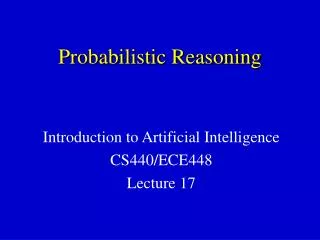
sensors environment ? agent actuators Temporal Probabilistic Agents t1, t2, t3, …
Time and Uncertainty • The world changes, we need to track and predict it • Examples: diabetes management, traffic monitoring • Basic idea: copy state and evidence variables for each time step • Xt – set of unobservable state variables at time t • e.g., BloodSugart, StomachContentst • Et – set of evidence variables at time t • e.g., MeasuredBloodSugart, PulseRatet, FoodEatent • Assumes discrete time step
States and Observations • Process of change is viewed as series of snapshots, each describing the state of the world at a particular time • Each time slice involves a set or random variables indexed by t: • the set of unobservable state variables Xt • the set of observable evidence variable Et • The observation at time t is Et = etfor some set of values et • The notation Xa:b denotes the set of variables from Xa to Xb
Markov processes Markov Assumption • Current state depends on only a finite history of previous states i.e. Xt depends on some bounded set of X0:t-1 First-order Markov process • P(Xt|X0:t-1) = P(Xt|Xt-1) Second-order Markov process • P(Xt|X0:t-1) = P(Xt|Xt-2, Xt-1)
Markov processes Sensor Markov assumption • P(Et|X0:t, E0:t-1) = P(Et|Xt) Assume stationary process • transition model P(Xt|Xt-1) and sensor model P(Et|Xt) are the same for all t • In a stationary process, the changes in the world state are governed by laws that do not themselves change over time
Complete Joint Distribution • Given: • Transition model: P(Xt|Xt-1) • Sensor model: P(Et|Xt) • Prior probability: P(X0) • Then we can specify complete joint distribution of over all variables :
Agenda • Temporal probabilistic agents • Inference: Filtering, prediction, smoothing and most likely explanation • Hidden Markov models • Kalman filters
Inference in Temporal Models • Having set up the structure of a generic temporal model, we can formulate the basic inference tasks that must be solved. • They are as follows: • Filtering or Monitoring • Prediction • Smoothing or Hindsight • Most likely explanation
Filtering or Monitoring • What is the probability that it is raining today, given all the umbrella observations up through today? • P(Xt|e1:t) - computing current belief state, given all evidence to date
Filtering or Monitoring Transition model Posterior distribution at time t Prediction Sensor model Filtering
Proof Dividing the evidence BayesRule Chain Rule Conditional Independence Marginal Probability Chain Rule Conditional Independence Forward Algorithm
Prediction • What is the probability that it will rain the day after tomorrow, given all the umbrella observations up through today? • P(Xt+k|e1:t) computing probability of some future state
Example • Let us illustrate the filtering process for two steps in the basic umbrella example • Assume that security guard has some prior belief as to whether it rained on day 0, just before the observation sequence begins. Let's suppose this is P(R0)=<0.5,0.5> • On day 1, the umbrella appears, so U1= true. The prediction from t=0 to t=1 is
Example … continued • Updating the evidence for t=1 gives • Prediction from t=1 to t=2 is • Updating the evidence for t=2 gives
Smoothing or Hindsight • What is the probability that it rained yesterday, given all the umbrella observations through today? • P(Xk|e1:t) 0 ≤ k < tcomputing probability of past state (hindsight)
Smoothing or Hindsight • Smoothing computes P(Xk|e1:t), the posterior distribution of the state at some past time k given a complete sequence of observations from 1 to t
Smoothing or Hindsight Dividing the evidence BayesRule Chain Rule Conditional Independence bk+1:t f1:k
Smoothing or Hindsight Sensor model Backward message at time k+1 Sensor model Backward Message at time k
Smoothing or Hindsight Marginal Probability BayesRule Chain Rule Conditional Independence Conditional Independence Backward Algorithm
Most likely explanation • If the umbrella appeared the first three days but not on the fourth, what is the most likely weather sequence to produce these umbrella sightings? • argmaxx1:xtP(x1:t|e1:t)given sequence of observation, find sequence of states that is most likely to have generated those observations.
Most likely explanation • Enumeration • Enumerate all possible state sequence • Compute the joint distribution and find the sequence with the maximum joint distribution • Smooth • Calculate the posterior distribution for each time step k • In each step k, find the state with maximum posterior distribution • Combine these states to form a sequence
Most likely explanation • Most likely path to each xt+1 = most likely path to some xt plus one more step • Identical to filtering except f1:t replaced by
Proof… Viterbi Algorithm Divide Evidence BayesRule Chain Rule Conditional Independence Chain Rule