Fronts and Frontogenesis

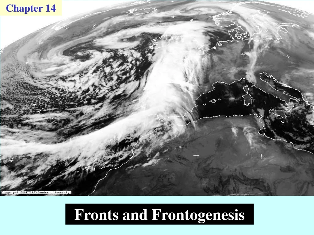
1. Chapter 14 Fronts and Frontogenesis

2. Satpix 1 IR Imagery 1200 06/04/2000

3. Satpix 2 WV Imagery 1200 06/04/2000

4. Problems with simple frontal models • Chapter 13 examines some simple air mass models of fronts and shows these to have certain deficiencies in relation to observed fronts. • Sawyer (1956) - "although the Norwegian system of frontal analysis has been generally accepted by weather forecasters since the 1920's, no satisfactory explanation has been given for the ‘up-gliding’ motion of the warm air to which is attributed the characteristic frontal cloud and rain. " • "Simple dynamical theory shows that a sloping discontinuity between two air masses with different densities and velocities can exist without vertical movement of either air mass...".

5. Sawyer => • "A front should be considered not so much as a stable area of strong temperature contrast between two air masses, but as an area into which active confluence of air currents of different temperature is taking place". q1 cold q1 Dy Dy q2 q2 warm

6. Several processes including friction, turbulence and vertical motion (ascent in warm air leads to cooling, subsidence in cold air leads to warming) might be expected to destroy the sharp temperature contrast of a front within a day or two of formation. • Clearly defined fronts are likely to be found only where active frontogenesis is in progress; i.e., in an area where the horizontal air movements are such as to intensify the horizontal temperature gradients. • These ideas are supported by observations.

7. The kinematics of frontogenesis Two basic horizontal flow configurations which can lead to frontogenesis: y y v(x) x x isotherms The intensification of a horizontal temperature gradient by (a) horizontal shear, and (b) a pure horizontal deformation field.

8. Relative motion near a point in a fluid Q u(x + dx, t) dx P u(x, t) O x In tensor notation summation over the suffix j is implied This decomposition is standard (see e.g. Batchelor, 1970, § 2.3)

9. It can be shown that eij and hij are second order tensors • eij is symmetric (eji = eij) • hijantisymmetric (hji = -hij ). • hij has only three non zero components and it can be shown that these form the components of the vorticity vector. Consider the case of two-dimensional motion Note: h11 = h22 =0

10. Write (x, y) = (xl, x2) and (du, dv) = (ul, u2) and take the origin of coordinates at the point P => (dxl, dx2) = (x, y). zis the vertical component of vorticity

11. In preference to the four derivatives vx, uy, vx, vy, define the equivalent four combinations of these derivatives: D = ux + vy,called the divergence E = ux- vycalled the stretching deformation F = vx+ uycalled the shearing deformation z = vx- uythe vorticity • E is called the stretching deformation because the velocity components are differentiated in the direction of the component. • F is called the shearing deformation because each velocity component is differentiated at right angles to its direction.

12. Obviously, we can solve for ux, vy, vx, vy as functions of D, E, F, z. Then may be written in matrix form as or in component form as

13. du = u - uo, dv = v - vo,and(uo, vo)is the translation velocity at the point P itself (now the origin). Choose the frame of reference so thatuo = vo = 0  du = u, dv = v. • The relative motion near the point P can be decomposed into four basic components as follows: • (I) Pure divergence(only D nonzero) • (II) Pure rotation (only z nonzero) • (III)Pure stretching deformation(only E nonzero) • (IV) Pure shearing deformation(only F nonzero).

14. (I)Pure divergence(only D nonzero) Pure divergence r is the position vector from P. P P D > 0 D < 0 The motion is purely radial and is from or to the point P according to the sign of D.

15. (II) Pure rotation (only z nonzero). Pure rotation u the unit normal vector to r r P The motion corresponds with solid body rotation with angular velocity .

16. (III)Pure stretching deformation(only E nonzero) On a streamline, dy/dx = v/u = -y/x , or xdy + ydx = d(xy) = 0. The streamlines are rectangular hyperbolae xy = constant. y streamlines for E > 0 axis of dilatation for E > 0 x axis of contraction for E > 0

17. (IV) Pure shearing deformation(only F nonzero) The streamlines are given now bydy/dx = x/y y y2- x2 = constant. The streamlines are again rectangular hyperbolae, but with their axes of dilatation and contraction at 45 degrees to the coordinate axes. 45o x The flow directions are for F > 0.

18. (V) Total deformation (only E and F nonzero) By rotating the axes(x, y)to(x', y')we can choosefso that the two deformation fields together reduce to a single deformation field with the axis of dilatation at anglefto the x axis. y y' x' f x

19. Let the components of any vector(a, b)in the(x, y)coordinates be(a', b')in the(x', y')coordinates: and where

20. where EandF, and also the total deformation matrices are not invariant under rotation of axes, unlike, for example, the matrices representing divergence and vorticity E'2 + F'2 = E2 + F2is invariant under rotation of axes. We can rotate the coordinate axes in such a way thatF' = 0; then E' is the sole deformation in this set of axes. tan 2f = F/E and

21. The stretching and shearing deformation fields may be combined to give atotal deformation field with strength E' and with the axis of dilatation inclined at an anglefto the x- axis. y axis of dilatation x axis of contraction

22. General two-dimensional motion near a point • In summary, the general two-dimensional motion in the neighbourhood of a point can be broken up into a field of divergence, a field of solid body rotation, and a single field of total deformation, characterized by its magnitude E' (> 0) and the orientation of the axis of dilatation, f. • We consider now how these flow field components act to change horizontal temperature gradients.

23. The frontogenesis function • One measure of the frontogenetic or frontolytic tendency in a flow is the frontogenesis function: • Start with the thermodynamic equation diabatic heat sources and sinks • Differentiating with respect to x and y in turn

24. and Now Note thatzdoes not appear on the right-hand-side! Use

25. There are four separate effects contributing to frontogenesis (or frontolysis): where unit vector in the direction of

26. . Interpretation T1 :represents the rate of frontogenesis due to a gradient of diabatic heating in the direction of the existing temperature gradient Cool Heat

27. T2 :represents the conversion of vertical temperature gradient to horizontal gradient by a component of differential vertical motion in the direction of the existing temperature gradient

28. T3 :represents the rate of increase of horizontal temperature gradient due to horizontal convergence (i.e., negative divergence) in the presence of an existing gradient

29. T4 :represents the frontogenetic effect of a (total) horizontal deformation field. • Further insight into this term may be obtained by a rotation of axes to those of the deformation field. • Let denote and relate to Solve for E and F in terms of E' and f(remember f is such that F' = 0)

30. y y` shq axis of dilatation x` g f x b axis of contraction Schematic frontogenetic effect of a horizontal deformation field on a horizontal temperature field.

31. shq Set x` a few lines of algebra g f x b angle between the axis of dilatation and the potential-temperature isotherms (isentropes) The frontogenetic effect of deformation is a maximum when the isentropes are parallel with the dilatation axis (b = 0), reducing to zero as the angle b between the isentropes and the dilatation axis increases to 45 deg. When the angle b is between 45 and 90 deg., deformation has a frontolytic effect, i.e., T4 < 0.

32. Observational studies • A number of observational studies have tried to determine the relative importance of the contributions Tn to the frontogenesis function. • Unfortunately, observational estimates of T2 are "noisy", since estimates for w tend to be noisy, let alone for shw. • T4 is also extremely difficult to estimate from observational data currently available. • A case study by Ogura and Portis (1982, see their Fig. 25) shows that T2, T3 and T4 are all important in the immediate vicinity of the front, whereas this and other investigations suggest that horizontal deformation (including horizontal shear) plays a primary role on the synoptic scale.

33. This importance is illustrated in Fig. 14.7, which is taken from a case study by Ogura and Portis (1982), and in Figs. 4.2 and 4.12, which show a typical summertime synoptic situation in the Australian region.

34. From a case study by Ogura and Portis (1982) surface front The direction of the dilatation axis and the resultant deformation on the 800 mb surface at 0200 GMT, 26 April 1979 with the contours of the 800 mb potential temperature field at the same time superimposed.

35. A mean sea level isobaric chart over Australia L H H H

36. A 1000-500 mb thickness chart over Australia H H H

37. In a study of many fronts over the British Isles, Sawyer (1956) found that ‘active’ fronts are associated with a deformation field which leads to an intensification of the horizontal temperature gradient. • He found also that the effect is most clearly defined at the 700 mb level at which the rate of contraction of fluid elements in the direction of the temperature gradient usually has a well-defined maximum near the front.

38. Flow deformation acting on a passive tracer to produce locally large tracer gradientsfrom Welander 1955

39. Dynamics of frontogenesis • The foregoing theory is concerned solely with the kinematics of frontogenesis and shows how particular flow patterns can lead to the intensification of horizontal temperature gradients. • We consider now the dynamical consequences of increased horizontal temperature gradients • We know that if the flow is quasi-geostrophic, these increased gradients must be associated with increased vertical shear through the thermal wind equation. • We show now by scale analysis that the quasi-geostrophic approximation is not wholly valid when frontal gradients become large, but the equations can still be simplified.

40. The following theory is based on the review article by Hoskins (1982). • It is observed, inter alia, that atmospheric fronts are marked by large cross-front gradients of velocity and temperature. • Assume that the curvature of the front is locally unimportant and choose axes with x in the cross-front direction, y in the along-front direction and z upwards: z y front x

41. Frontal scales and coordinates V cold warm L v y uh u U x l

42. Observations show that typically, • U ~ 2 ms -1 • V ~ 20 ms -1 • L 1000 km • l ~ 200 km • => V >> UandL >> l. • The Rossby number for the front, defined as is typically of order unity. The relative vorticity (~V/l) is comparable with f and the motion is not quasi-geostrophic.

43. The ratio of inertial to Coriolis accelerations in the x and y directions => and The motion is quasi -geostrophic across the front, but not along it. A more detailed scale analysis is presented by Hoskins and Bretherton (1972, p15), starting with the equations in orthogonal curvilinear coordinates orientated along and normal to the surface front.

44. The scale analysis, the result of Exercise (14.3), and making the Boussinesq approximation, the equations of motion for a front are buoyancy force per unit mass N0 = the Brunt-Väisälä frequency of the basic state • I assume that f and N0 are constants.

45. Quasi-geostrophic frontogenesis • While the scale analysis shows that frontal motions are not quasi-geostrophic overall, much insight into frontal dynamics may be acquired from a study of frontogenesis within quasi-geostrophic theory. • Such a study provides also a framework in which later modifications, relaxing the quasi-geostrophic assumption, may be better appreciated.

46. The quasi-geostrophic approximation involves replacing D/Dt by where vg = v is computed from fv = xP as it stands and Set u = ug + ua and

47. fvz = sx

48. Let us consider the maintenance of cross-front thermal wind balance expressed by fvz = sx. Note that ugx + vy = 0 These equations describe how the geostrophic velocity field acting through Qlattempts to destroy thermal wind balance by changing fvz and sx by equal and opposite amounts and how ageostrophic motions (ua, w) come to the rescue!

49. Also from uax + wz = 0, there exists a streamfunctiony for the cross-frontal circulation satisfying This is a Poisson-type elliptic partial differential equation for the cross-frontal circulation, a circulation which is forced by Ql.

50. Membrane analogy for solving a Poisson Equation This is an Elliptic PDE F > 0 Here z = 0 on the domain boundary F < 0 This is called a Dirichlet condition