Title
Understand relative calibration methods for seismometers, importance of frequency response analysis, and practical techniques for accurate results. Learn about signal modeling, geophone calibration, and digitizer calibrations in this informative training course.

Title
E N D
Presentation Transcript
Title International Training Course, Rabat 2012 E. Wielandt: Relative (electrical) calibration of seismometers
Systematics Recorded? Assumed?
Relative calibration (determining the frequency response) A variety of signals - sinewaves, pulses, pseudo-random signals - can be used for seismometer calibration. However, it is risky to rely on the precision of a waveform generator. Preferably, the input signal should be recorded together with the output signal. The transfer function is defined as the complex gain for sinewaves, but in order to make practical use of this relationship, one must wait for a steady state after each change of the frequency. This is not practical for broadband seismometers. Also, we want a mathematical representation of the response, not a table for discrete frequenies. Modelling the output signal from the input signal (preferably in time domain), and matching the parameters of the mathematical model, is a more efficient method of determining the frequency response. Text
Simplest but not best: measuring the amplitude response of a geophone to sinewaves
By superimposing standardized response curves,the parameters can be directly determined ( 4.5 Hz geophone with 0.4 of crit. damping)
Resonance curves can of course be fitted automatically, and even the exact frequency of the sinewaves can be determined from the record. The only requirement is that the input sinewaves all have the same amplitude. This method is quite useful for the remote calibration of geophone-type sensors. The next slide shows the output signal from which the constants of a Geotech S13 in the GERESS array were determined with the SINCAL routine (download) as:. T0 = 0.979 s, h = 0.774 Text
SINCAL2 best fit boots.avg. std.dev. Period 0.932 0.932 +- 0.000 Damping 0.7481 0.7479 +- 0.0006 Gain 1503.96 1503.84 +- 0.68 sincal
If the geophone has no calibration coil, then the signal coil can be used for both input and output. The voltage across the coil caused by the input current can later be automatically subtracted from the output (program CALEX3, download). halfbridge
Calibration of a 10 Hz field geophone with a half-bridge, using a squarewave as an input. From top: input current, recorded output voltage, modeled output voltage, misfit. Note that the misfit is not the same for the mass jumping „up“ and „down“, indicating a dependence of the free period on mass position, i.e. a nonlinearity.Such problems can only be recognized in time domain. 10 Hz geophone
Hardware used for calibration with a logarithmic sweep. The left box splits the signal into adjustable U, V, W components for the STS2, and can deliver purely „horizontal“ or „vertical“ calibration signals.
It is also possible to calibrate the U, V, and W sensors separately - the Z output may be used for this purpose - and then to average the U, V, W transfer functions or parameters with a matrix whose elements are the squares of those of the matrix transforming the U, V, W into the X, Y, Z components:
Calibration of an STS2 seismometer with a sweep signal from 20 s to 400 s period. The rms residual is only 1/3000 of the rms output signal, and consists mainly of ambient long-period noise. a sweep calibration
Another example. The sweep this time covers a band from 20 s to 800 s. The relatively large and strange-looking residual is caused by a defective 16-bit digitizer that produces a small jump in every zero crossing. Time-domain modelling with the CALEX method helps to identify such problems. another sweep calibration
Calibration of Digitizers • Digitizers normally don’t need to be calibrated if the manufacturer’s specifications are clear and complete. • You may want to check the scale factor, normally in microvolts per count, by connecting a battery and a digital voltmeter to the input. • Forget about the filter coefficients! You only need to know the filter type (minimum-delay or zero-phase). • For all frequencies lower than one-quarter of the sampling rate, (that is, one-half of the Nyquist bandwith) you may assume that the response is flat and the phase: • of a zero-phase filter is zero • of a minimum-delay filter represents a constant delay whose magnitude you can experimentally determine by recording a time signal (such as from the pps output of a GPS receiver). At low frequencies, even a minimum-delay filter is nearly linear-phase (but not zero-phase). • - You should also check if the delay of a zero-phase filter is really zero. There might be an error in the time-tag.
„Minimum phase“ is normally maximum phase The term „minimum phase“ was coined with respect to a Fourier transformation with exp(jwt) in the forward transformation. Most seismologists use however exp(-jwt). Then the signal with the smallest possible delay – the minimum-delay signal – has, mathematically speaking, the largest possible (although negative) phase. The unambiguous term „minimum-delay“ is preferable to the term „minimum-phase“.