Automated Reasoning

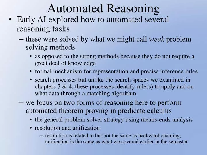
1. Automated Reasoning • Early AI explored how to automated several reasoning tasks • these were solved by what we might call weak problem solving methods • as opposed to the strong methods because they do not require a great deal of knowledge • formal mechanism for representation and precise inference rules • search processes but unlike the search spaces we examined in chapters 3 & 4, these processes identify rule(s) to apply and on what data through a matching algorithm • we focus on two forms of reasoning here to perform automated theorem proving in predicate calculus • the general problem solver strategy using means-ends analysis • resolution and unification • resolution is related to but not the same as backward chaining, unification is the same as what we covered earlier in the semester

2. Theorem Proving • We first examine the Logic Theorist system, built in 1956 by (Allen) Newell, Shaw and Simon • given two statements in propositional calculus, it would try to prove their equality • it would use a collection of rules (shown in a few slides) • LT’s rules performed one of three types of operations • substitution – substitute one expression for every occurrence of a symbol that is already known to be true • (B v B)  B can be replaced by (!A v !A)  !A or by ((C*D*!E v C*D*!E)  C*D*!E) • replacement – substitute an expression that has a connective (e.g., ) by its equivalent form or definition • A  B can be replaced by !A v B since they are equivalent • detachment – apply modus ponens to introduce a new, true statement or clause

3. Means-Ends Analysis, GPS and LT • Means-ends analysis – weak method approach • compare current state to goal state to determine differences • select an operator to reduce some of these differences • a difference table is set up that shows how, for every operator, it impacts the differences • GPS is the general problem solver, a system that embodies this weak method approach • GPS is a generalized version of the process used in LT • LT is given two logical statements, the first is the start state and the second is the goal state, and LT attempts to show their equivalence by reducing one into the other • differences are determined using a difference table consisting of actions to either reduce a term, add a term, or change a term including • changes in sign (AND to OR, OR to AND) and connective ( to OR) • the rules to apply (there were 12 of them) would all be based on Boolean algebra laws such as DeMorgan’s Law

4. How LT Works • LT applies inference rules in a breadth-first, goal-driven manner, using four methods • substitute a symbol in the current goal to see if it matches any known axiom or theorem, if so, that goal has been proved • try all possible detachments and replacements to the goal • test each generated term using substitution • any that fail to prove the goal are added to a subproblem list • employ transitivity of implication to see if it would solve the problem and if so, add the new term as a new subprogram • e.g., if we are trying to prove AC and we know BC, then we add AB, if we can prove that is true, then we have proven AC • if known of the above work, remove the first term off the subproblem list and repeat with this as the goal

5. LT Rules and Examples If we have (X * Y), by rule 1, we can change this to (Y * X) If we have X * Y  !Z, by rule 2, we can change this to !(X * Y) v !!Z and then apply rule 5 and double negation to obtain !X v !Y v Z If we know X is true and !Y is true, we can use rule 10 to obtain X * !Y If we need to have X, and we know A and B are true and (A & B)  (X & Y), we can use rules 10, 11 and 8 to obtain X

6. How Does LT Select a Rule? • LT uses subgoaling to solve its problem • given a goal, use means-ends analysis to determine the difference between the goal and the current state • next, select a rule to reduce this difference • if the rule can reduce the difference directly, great, otherwise produce a subgoal and add it to the list of goals/subgoals • LT uses a difference reduction table to determine which rule(s) of the 12 rules can be used to accomplish the given difference • for instance, to delete a term, use rule 3, 7, 8, 11 or 12 and to change a sign, use rule 5

7. Example Goals and Strategies

8. Resolution • When we first examined first order predicate calculus, we used our representation by applying chaining, modus ponens and unification • another way to use predicate calculus is resolution and unification • In resolution, introduce the negation of what you want to prove into your knowledge base • in first order predicate calculus, everything known fact is true • you have assumed the new piece of knowledge is true • now, resolve terms by combining terms by AND-ing them • this creates a new term in which some element of the previous term may be canceled out • if you have (X v Y), !X and AND them together, you get Y • add unification as necessary • In resolution, if you can reduce your terms to the empty clause (cancel out all terms) then you have an inconsistency • either your original knowledge base was wrong (we assume not) or the new term is wrong • if the new term is wrong, then its opposite must be true, therefore if you introduced !X then X must be true, you have proved it X

9. Clausal Form • To use resolution, you must translate your knowledge into predicate calculus statements and then into clausal form • eliminate  by using the equivalent form • A  B = !A v B • reduce negation so that it appears immediately before predicates, not terms by applying DeMorgan’s Law • also Double Negation, or by moving from prior to the quantifier to immediately before the term (see page 586) • remove any universal quantifiers by renaming variables • if you have for all x:… for all x: …, change the latter grouping into y • remove any existential quantifiers by replacing the variables with constants • convert all clauses to be conjuncts of disjuncts • each term should consist of only ANDs, ORs, and NOTs • arrange them so that they are ORed items of individual predicates or of ANDed predicates: A*B v !B*C*D v !A • separate each conjunct into its own term – these terms will only comprise predicates, NOTs and ORs in some combination • Now, introduce the negation of what you want to prove • see the notes for some examples

10. Question Answering • Given a KB with knowledge of specific instances, we can also use resolution to pose a question • e.g., who is ready to graduate? • The process is almost identical to our previous resolution where we tried to prove something was true • here, we introduce the negation of the question we want to answer (e.g., ~ready_to_graduate(X)) • through unification, we are hoping to find an X that makes the above statement false, and therefore the person that we unified to X is ready to graduate • this process can only work by having instances that can unify to the term that we are attempting to prove • the answer is the instance(s) that unified to X • in the Prolog language, the system will find all X’s but in resolution, we usually stop when we have found an X • again, see the notes for an example

11. Clause Selection Strategies • As with our previous AI solutions, resolution is search based • which clause should we select to attempt to resolve? • what instance do we unify with a variable? • so resolution/unification is intractable (too computationally complex) • There are many different approaches to tackling the search problem • breadth-first – while this strategy computationally is poor because it generates all possible solution spaces until one is found, the proof itself will take the fewest steps • depth-first – this strategy may “luck” into a solution much quicker than breadth-first and is easy to implement using recursion • We can also use one or more heuristic approaches • support – select a clause to unify where one of the terms is related to a term to be resolved (related in terms of hierarchical) • unit preference – select a clause with the fewest terms (1 preferably) • linear input – always select a clause that has the negation of at least one term in the resolvent – that is, make sure you are always removing clauses as you go