
Geant4 optics
E N D
Presentation Transcript
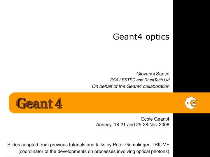
Geant4 optics Giovanni Santin ESA / ESTEC and RheaTech Ltd On behalf of the Geant4 collaboration Ecole Geant4 Annecy, 18-21 and 25-28 Nov 2008 Slides adapted from previous tutorials and talks by Peter Gumplinger, TRIUMF (coordinator of the developments on processes involving optical photons)
Outline • Introduction • Optical processes • Processes producing photons • Processes undergone by photons • Optical properties in material property tables • Examples Giovanni Santin - General Particle Source (GPS) - Ecole Geant4 2008, Annecy
Optical photons Introduction Basic functioning Position, angular & energy distributions Examples • Physically optical photons should be covered by the electromagnetic category, but • optical photon wavelength is >> atomic spacing • treated as waves no smooth transition between optical and gamma particle classes • G4OpticalPhoton: wave like nature of EM radiation • G4OpticalPhoton <=|=> G4Gamma • New particle type • No smooth transition // optical photon G4OpticalPhoton::OpticalPhoton(); • Define a (spin) vector for the photon, added as data member to the G4DynamicParticle description class aphoton->SetPolarization(ux,uy,uz); // unit vector!!! /gps/polarization ux uy uz /gun/polarization ux uy uz Giovanni Santin - General Particle Source (GPS) - Ecole Geant4 2008, Annecy
Optical properties associated to G4Material • Optical properties can be specified as properties table in G4Material • reflectivity, transmission efficiency, dielectric constants, surface properties • Photon spectrum properties also defined in G4Material • scintillation yield, time structure (fast, slow components) • Properties are expressed as a function of the photon’s momentum const G4int NUMENTRIES = 32; G4double photmom[NUMENTRIES] = {2.034*eV, ……, 4.136*eV}; G4double rindex[NUMENTRIES] = {1.3435, ……, 1.3608}; G4double absorption[NUMENTRIES] = {344.8*cm, ……, 1450.0*cm}; G4MaterialPropertiesTable *MPT = new G4MaterialPropertiesTable(); MPT -> AddProperty(“RINDEX”,photmom,rindex,NUMENTRIES}; MPT -> AddProperty(“ABSLENGTH”,photmom,absorption,NUMENTRIES}; G4NistManager* man = G4NistManager::Instance(); G4Material* water = man->FindOrBuildMaterial("G4_WATER"); water -> SetMaterialPropertiesTable(MPT); Giovanni Santin - General Particle Source (GPS) - Ecole Geant4 2008, Annecy
Processes producing optical photons • Optical photons are produced by the following Geant4 processes: • G4Cerenkov • G4Scintillation • G4TransitionRadiation • Classes located in processes/electromagnetic/xrays • Warning: these processes generate optical photons without energy conservation Giovanni Santin - General Particle Source (GPS) - Ecole Geant4 2008, Annecy
Cerenkov Process • Cerenkov light occurs when a charged particle moves through a medium faster than the medium’s group velocity of light. • Photons are emitted on the surface of a cone, and as the particle slows down: • the cone angle decreases • the emitted photon frequency increases • and their number decreases • Cerenkov photons have inherent polarization perpendicular to the cone’s surface. Giovanni Santin - General Particle Source (GPS) - Ecole Geant4 2008, Annecy
G4Cerenkov Implementation Details • Cerenkov photon origins are distributed rectilinear over the step even in the presence of a magnetic field • Cerenkov photons are generated only in media where the user has provided an index of refraction • An average number of photon is calculated for the wavelength interval in which the index of refraction is given • New: Cerenkov photon number varies linearly with velocity (no longer uniformly distributed along the step) Giovanni Santin - General Particle Source (GPS) - Ecole Geant4 2008, Annecy
G4CerenkovUser options • Suspend primary particle and track Cerenkov photons first • e.g. to avoid tracking all photons if the event is globally not interesting • Set the (max) average number of Cerenkov photons per step • The actual number generated in any given step will be slightly different because of the statistical nature of the process • example ExptPhysicsList: #include “G4Cerenkov.hh” G4Cerenkov* theCkovProcess = new G4Cerenkov(“Cerenkov”); theCkovProcess -> SetTrackSecondariesFirst(true); G4int MaxNumPhotons = 300; theCkovProcess->SetMaxNumPhotonsPerStep(MaxNumPhotons); • G4Cerenkov can limit the Step by: • User defined average maximum number of photons to be generated during a step • New: User defined maximum allowed change in beta = v/c in % during the step. • New: A definite step limit when the track drops below the Cerenkov threshold Giovanni Santin - General Particle Source (GPS) - Ecole Geant4 2008, Annecy
Scintillation process • Number of photons generated proportional to the energy lost during the step • Emission spectrum sampled from empirical spectra • Isotropic emission • Uniform along the track segment • With random linear polarization • Emission time spectra with one exponential decay time constant Giovanni Santin - General Particle Source (GPS) - Ecole Geant4 2008, Annecy
Scintillation material has a characteristic light yield The statistical yield fluctuation is either broadened due to impurities for doped crystals or narrower as a result of the Fano Factor Suspend primary particle and track scintillation photons first Example physics list: #include “G4Scintillation.hh” G4Scintillation* theScintProcess = new G4Scintillation(“Scintillation”); theScintProcess -> SetTrackSecondariesFirst(true); theScintProcess -> SetScintillationYieldFactor(0.2); theScintProcess -> SetScintillationExcitationRatio(1.0); Note The ‘YieldFactor’ allows for different scintillation yields depending on the particle type In such case, separate scintillation processes must be attached to the various particles G4ScintillationProcess implementation details Giovanni Santin - General Particle Source (GPS) - Ecole Geant4 2008, Annecy
G4Scintillation details: material properties #include “G4Material.hh // Liquid Xenon material G4Element* elementXe = new G4Element(“Xenon”,”Xe”,54.,131.29*g/mole); G4Material* LXe = new G4Material (“LXe”,3.02*g/cm3,1, kStateLiquid, 173.15*kelvin, 1.5*atmosphere); LXe -> AddElement(elementXe, 1); const G4int NUMENTRIES = 9; G4double LXe_PP[NUMENTRIES] = {6.6*eV,6.7*eV,6.8*eV,6.9*eV,7.0*eV, 7.1*eV,7.2*eV,7.3*eV,7.4*eV}; G4double LXe_SCINT[NUMENTRIES] = {0.000134, 0.004432, 0.053991, 0.241971, 0.398942, 0.000134, 0.004432, 0.053991,0.241971}; G4double LXe_RIND[NUMENTRIES] = { 1.57, 1.57, 1.57, 1.57, 1.57, 1.57, 1.57, 1.57, 1.57}; G4double LXe_ABSL[NUMENTRIES] = { 35.*cm, 35.*cm, 35.*cm, 35.*cm, 35.*cm, 35.*cm, 35.*cm, 35.*cm, 35*cm }; G4MaterialPropertiesTable* LXe_MPT = new G4MaterialPropertiesTable(); LXe_MPT -> AddProperty(“FASTCOMPONENT”,LXe_PP,LXe_SCINT,NUMENTRIES); LXe_MPT -> AddProperty(“RINDEX”, LXe_PP,LXe_RIND,NUMENTRIES); LXe_MPT -> AddProperty(“ABSLENGTH”,LXe_PP, LXe_ABSL,NUMENTRIES); LXe_MPT -> AddConstProperty (“SCINTILLATIONYIELD”, 100./MeV); LXe_MPT -> AddConstProperty(“RESOLUTIONSCALE”,1.0) LXe_MPT -> AddConstProperty(“FASTTIMECONSTANT”,45.*ns); LXe_MPT -> AddConstProperty(“YIELDRATIO”,1.0); LXe -> SetMaterialPropertiesTable(LXe_MPT); Giovanni Santin - General Particle Source (GPS) - Ecole Geant4 2008, Annecy
Processes undergone by optical photons • Optical photons undergo: • bulk absorption • Rayleigh scattering • wavelength shifting • refraction and reflection at medium boundaries • Classes located in processes/optical • Geant4 keeps track of polarization • but not overall phase no interference • ExampleN06 at examples/novice/N06 Giovanni Santin - General Particle Source (GPS) - Ecole Geant4 2008, Annecy
G4OpAbsorption • Bulk absorption • uses photon attenuation length from material properties to get mean free path • photon is simply killed after a selected path length G4double PhotonEnergy[nEntries] = {6.6*eV,6.7*eV,6.8*eV,6.9*eV,7.0*eV,7.1*eV,7.2*eV,7.3*eV,7.4*eV}; G4double AbsLength[nEntries] = {0.1*mm,0.2*mm,0.3*mm,0.4*cm,1.0*cm,10.0*cm,1.0*m,10.0*m,10.0*m}; MPT->AddProperty(“ABSLENGTH”,PhotonEnergy,AbsLength,NUMENTRIES}; Giovanni Santin - General Particle Source (GPS) - Ecole Geant4 2008, Annecy
Rayleigh ScatteringG4OpRayleigh • Elastic scattering including polarization of initial and final photons • The scattered photon direction is perpendicular to the new photon polarization in such a way that the final direction, initial and final polarization are all in one plane • The diff. cross section is proportional to cos2(a) where a is the angle between the initial and final photon polarization • Rayleigh scattering attenuation coefficient is calculated for “Water” material following the Einstein-Smoluchowski formula, but in all other cases it must be provided by the user: MPT -> AddProperty(“RAYLEIGH”,PhotonEnergy,Scattering,NUMENTRIES}; Giovanni Santin - General Particle Source (GPS) - Ecole Geant4 2008, Annecy
Wavelength shifting • Handled by G4OpWLS • initial photon is killed, one with new wavelength is created • builds it own physics table for mean free path • User must supply: • Absorption length as function of photon energy • Isotropic emission • With random linear polarization • Emission spectra parameters as function of energy • Possible time delay between absorption and re-emission Giovanni Santin - General Particle Source (GPS) - Ecole Geant4 2008, Annecy
Wavelength-shifting: example code #include “G4Material.hh const G4int nEntries = 9; G4double PhotonEnergy[nEntries] = {6.6*eV,6.7*eV,6.8*eV,6.9*eV,7.0*eV,7.1*eV,7.2*eV,7.3*eV,7.4*eV}; G4double RIndexFiber[nEntries] = {1.6, 1.6, 1.6, 1.6, 1.6, 1.6, 1.6, 1.6, 1.6}; G4double AbsFiber[nEntries] = {0.1*mm,0.2*mm,0.3*mm,0.4*cm,1.0*cm,10.0*cm,1.0*m,10.0*m,10.0*m}; G4double EmissionFiber[nEntries] = {0.0, 0.0, 0.0, 0.1, 0.5, 1.0, 5.0, 10.0, 10.0}; G4Material* WLSFiber; G4MaterialPropertiesTable* MPTFiber = new G4MaterialPropertiesTable(); MPTFiber->AddProperty(“RINDEX”, PhotonEnergy,RIndexFiber,nEntries); MPTFiber->AddProperty(“WLSABSLENGTH”,PhotonEnergy,AbsFiber,nEntries); MPTFiber->AddProperty(“WLSCOMPONENT”,PhotonEnergy,EmissionFiber,nEntries); MPTFiber->AddConstProperty (“WLSTIMECONSTANT”, 0.5*ns); WLSFiber->SetMaterialPropertiesTable(MPTFiber); Giovanni Santin - General Particle Source (GPS) - Ecole Geant4 2008, Annecy
Boundary processes Giovanni Santin - General Particle Source (GPS) - Ecole Geant4 2008, Annecy
Boundary interactionsOptical photons as particles • Geant4 demands particle-like behavior for tracking: • thus, no “splitting” • event with both refraction and reflection must be simulated by at least two events Giovanni Santin - General Particle Source (GPS) - Ecole Geant4 2008, Annecy
Handled by G4OpBoundaryProcess refraction reflection User must supply surface properties using G4OpticalSurface models Boundary properties dielectric-dielectric dielectric-metal dielectric-black material Surface properties: polished ground front- or back-painted, ... Boundary interactions Giovanni Santin - General Particle Source (GPS) - Ecole Geant4 2008, Annecy
Boundary Step Post-step point Pre-step point G4BoundaryProcessImplementation Details • A ‘discrete process’, called at the end of every step • Never limits the step (done by the transportation) • Sets the ‘forced’ condition • Logic such that • preStepPoint: is still in the old volume • postStepPoint: is already in the new volume so information is available from both Giovanni Santin - General Particle Source (GPS) - Ecole Geant4 2008, Annecy
Surface Concept Split into two classes • Conceptual class: G4LogicalSurface (in the geometry category) holds • pointers to the relevant physical or logical volumes • pointer to a G4OpticalSurface These classes are stored in a table and can be retrieved by specifying: • an ordered pair of physical volumes touching at the surface [G4LogicalBorderSurface] • in principle allows for different properties depending on which direction the photon arrives • or a logical volume entirely surrounded by this surface [G4LogicalSkinSurface] • useful when the volume is coded by a reflector and placed into many volumes • limitation: only one and the same optical property for all the enclosed volume’s sides) • Physical class: G4OpticalSurface (in the material category) keeps information about the physical properties of the surface itself Giovanni Santin - General Particle Source (GPS) - Ecole Geant4 2008, Annecy
G4OpticalSurface • Set the simulation model used by the boundary process: • GLISUR-Model: original G3 model • UNIFIED-Model: adopted from DETECT (TRIUMF) enum G4OpticalSurfaceModel {glisur, unfied}; • Set the type of interface: enum G4OpticalSurfaceType { dielectric_metal, dielectric_dielectric}; • Set the surface finish: enum G4OpticalSurfaceFinish { polished, // smooth perfectly polished surface polishedfrontpainted, // polished top-layer paint polishedbackpainted, // polished (back) paint/foil ground, // rough surface groundfrontpainted, // rough top-layer paint groundbackpainted // rough (back) paint/foil }; Giovanni Santin - General Particle Source (GPS) - Ecole Geant4 2008, Annecy
Optical surface types • Dielectric - Dielectric Depending on the photon’s wave length, angle of incidence, (linear) polarization, and (user input) refractive index on both sides of the boundary: • total internal reflected • Fresnel refracted • Fresnel reflected • Dielectric – Metal The photon cannot be transmitted. • absorbed (detected), with probability estimated according to the table provided by the user • reflected • Dielectric – Black material A black material is a tracking medium for which the user has not defined any optical property. The photon is immediately absorbed undetected Giovanni Santin - General Particle Source (GPS) - Ecole Geant4 2008, Annecy
Surface effects • POLISHED: In the case where the surface between two bodies is perfectly polished, the normal used by the G4BoundaryProcess is the normal to the surface defined by: • the daughter solid entered; or else • the solid being left behind • GROUND: The incidence of a photon upon a rough surface requires choosing the angle, a, between a ‘micro-facet’ normal and that of the average surface. • The UNIFIED model assumes that the probability of micro-facet normals that populates the annulus of solid angle sin(a)da will be proportional to a gaussian of SigmaAlpha: theOpSurface -> SetSigmaAlpha(0.1); [rad] • In the GLISUR model this is indicated by the value of polish; when it is <1, then a random point is generated in a sphere of radius (1-polish), and the corresponding vector is added to the normal. The value 0 means maximum roughness with effective plane of reflection distributed as cos(a). theOpSurface -> SetPolish(0.0); • The ‘facet normal’ is accepted if the refracted wave is still inside the original volume. Giovanni Santin - General Particle Source (GPS) - Ecole Geant4 2008, Annecy
Microfacets • The assumption is that a rough surface is a collection of ‘microfacets’ Giovanni Santin - General Particle Source (GPS) - Ecole Geant4 2008, Annecy
In cases (b) and (c), multiple interactions with the boundary are possible within the process itself and without the need for relocation by the G4Navigator. Giovanni Santin - General Particle Source (GPS) - Ecole Geant4 2008, Annecy
Csl: Reflection prob. about the normal of a micro facet • Css: Reflection prob. about the average surface normal • Cdl: Prob. of internal Lambertian reflection • Cbs: Prob. of reflection within a deep grove with the ultimate result of exact back scattering. Giovanni Santin - General Particle Source (GPS) - Ecole Geant4 2008, Annecy
The G4OpticalSurface also has a pointer to a G4MaterialPropertiesTable • In case the surface is painted, wrapped, or has a cladding, the table may include the thin layer’s index of refraction • This allows the simulation of boundary effects both • at the intersection between the medium and the surface layer and • at the far side of the thin layer all within the process itself and without invoking the G4Navigator • the thin layer does not have to be defined as a G4 tracking volume Giovanni Santin - General Particle Source (GPS) - Ecole Geant4 2008, Annecy
Example G4LogicalVolume * volume_log; G4VPhysicalVolume * volume1; G4VPhysicalVolume * volume2; // Surfaces G4OpticalSurface* OpWaterSurface = new G4OpticalSurface(“WaterSurface”); OpWaterSurface -> SetModel(glisur); OpWaterSurface -> SetType(dielectric_metal); OpWaterSurface -> SetFinish(polished); G4LogicalBorderSurface* WaterSurface = new G4LogicalBorderSurface(“WaterSurface”,volume1,volume2,OpWaterSurface); G4OpticalSurface * OpAirSurface = new G4OpticalSurface(“AirSurface”); OpAirSurface -> SetModel(unified); OpAirSurface -> SetType(dielectric_dielectric); OpAirSurface -> SetFinish(ground); G4LogicalSkinSurface * AirSurface = new G4LogicalSkinSurface(“AirSurface”,volume_log,OpAirSurface); Giovanni Santin - General Particle Source (GPS) - Ecole Geant4 2008, Annecy
Example (2) G4OpticalSurface * OpWaterSurface = new G4OpticalSurface(“WaterSurface”); OpWaterSurface -> SetModel(unified); OpWaterSurface -> SetType(dielectric_dielectric); OpWaterSurface -> SetFinish(groundbackpainted); Const G4int NUM = 2; G4double pp[NUM] = {2.038*eV, 4.144*eV}; G4double specularlobe[NUM] = {0.3, 0.3}; G4double specularspike[NUM] = {0.2, 0.2}; G4double backscatter[NUM] = {0.1, 0.1}; G4double rindex[NUM] = {1.35, 1.40}; G4double reflectivity[NUM] = {0.3, 0.5}; G4double efficiency[NUM] = {0.8, 1.0}; G4MaterialPropertiesTable *SMPT = new G4MaterialPropertiesTable(); SMPT -> AddProperty(“RINDEX”, pp, rindex, NUM); SMPT -> AddProperty(“SPECULARLOBECONSTANT”,pp,specularlobe,NUM); SMPT -> AddProperty(“SPECULARSPIKECONSTANT”,pp,specularspike,NUM); SMPT -> AddProperty(“BACKSCATTERCONSTANT”,pp,backscatter,NUM); SMPT -> AddProperty(“REFLECTIVITY”,pp,reflectivity,NUM); SMPT -> AddProperty(“EFFICIENCY”,pp,efficiency,NUM); OpWaterSurface -> SetMaterialPropertiesTable(SMPT); Giovanni Santin - General Particle Source (GPS) - Ecole Geant4 2008, Annecy
Logic in G4OpBoundaryProcess:PostStepDoIt • Make sure: • the photon is at a boundary (StepStatus = fGeomBoundary) • the last step taken is not a very short step (StepLength>=kCarTolerance/2) as it can happen upon reflection ELSE do nothing and RETURN • If the two media on either side are identical do nothing and RETURN • If the original medium had no G4MaterialPropertiesTable defined kill the photon and RETURN ELSE get the refractive index • Get the refractive index for the medium on the other side of the boundary, if there is one • See, if a G4LogicalSurface is defined between the two volumes if so get the G4OpticalSurface which contains physical surface parameters • Default to glisur model and polished surface • If the new medium had a refractive index, set the surface type to ‘dielectric-dielectric’ ELSEIF get the refractive index from the G4OpticalSurface ELSE kill the photon • Use (as far as it has the information) G4OpticalSurface to model the surface ELSE use Default Giovanni Santin - General Particle Source (GPS) - Ecole Geant4 2008, Annecy
As a consequence • For polished interfaces, no ‘surface’ is needed if the index of refraction of the two media is defined • The boundary process implementation is rigid about what it expects the G4Navigator does upon reflection on a boundary • G4BoundaryProcess with ‘surfaces’ is only possible for volumes that have been positioned by using placement rather than replica or touchables Giovanni Santin - General Particle Source (GPS) - Ecole Geant4 2008, Annecy
Examples • Some user applications • N06 • examples/novice/N06 • Liquid Xenon • examples/extended/optical/LXe Giovanni Santin - General Particle Source (GPS) - Ecole Geant4 2008, Annecy
Sample of user applications Courtesy A. Etenko, I. Machulin - Kurchatov Institute Courtesy H.Araujo (Imperial College London & UK Dark Matter Collaboration) G.Santin, HARP Cerenkov, CERN Giovanni Santin - General Particle Source (GPS) - Ecole Geant4 2008, Annecy
ExampleN06 Giovanni Santin - General Particle Source (GPS) - Ecole Geant4 2008, Annecy
Giovanni Santin - General Particle Source (GPS) - Ecole Geant4 2008, Annecy
Summary • Optical processes handle • the reflection, refraction, absorption, wavelength shifting and scattering of long-wavelength photons, and • the productions of photons by scintillation, Cerenkov and transition radiation • The simulation may commence with the propagation of a charged particle and end with the detection of the ensuing optical photons on photo sensitive areas, all within the same event loop • Documentation http://cern.ch/geant4 User support Application Developers Guide Optical photon processes http://cern.ch/geant4 User support Physics reference manual Optical photons • Examples • examples/novice/N06 • examples/extended/optical/LXe • Forum http://cern.ch/geant4 User support User forum Processes Involving Optical Photons Giovanni Santin - General Particle Source (GPS) - Ecole Geant4 2008, Annecy