Download
1 / 14
140 likes | 290 Views
Methods of Detecting the Gravitational Wave Background. A pilgrimage in statistics 12th December, 2007 Daniel Yardley. Collaborators. Bill Coles - stats guru George Hobbs - software/simulations guru Rest of PPTA team (more gurus)…. George getting hit by a gravitational wave. Outline.

E N D
Methods of Detecting the Gravitational Wave Background A pilgrimage in statistics 12th December, 2007 Daniel Yardley
Collaborators • Bill Coles - stats guru • George Hobbs - software/simulations guru • Rest of PPTA team (more gurus)…
Outline • Why measure correlations? • What do we expect (hope) to see? • Issues with calculating correlations. • Simulations, analysis code and results.
Why Correlation? • Removes many sources of noise. • Gives many more samples than pulsars • Gives possibility of direct detection of isotropic stochastic GW background in shorter time than single pulsar. • Chosen GWB is
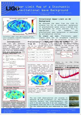
Previous Method (Jenet): Find correlation between expected theoretical curve and measured correlations. New Method (Coles) Do a least-squares fit between measured correlations and expected curve scaled by g2, variance of GW-induced residuals Gives us GW Amplitude A also. Significance of Detection
Issues and Techniques • Smoothing - enables us to reach max sensitivity at lower SNR • Pre-whitening (requires regular sampling) - dramatically increases max sensitivity. This must be done for PPTA project (or PPTA program (M Kramer’s suggestion) ). Increases number of degrees of freedom in data by flattening the steep red power spectra.
Frequency Domain Techniques • Cross power spectra: x1(t) and x2(t) data sets, then CP spectrum will be • Best estimate of covariance obtained by using a weighted sum over f: • Optimal weight factors: flattens spectrum where GWB dominates; culls spectrum where noise dominates
Simulations and Code • Simulate pulsar data sets and GW backgrounds using TEMPO2. • Analysis code: interpolate pulsar data to daily sampling, take every 14th point for biweekly sampling - gives evenly sampled data set. Make power spectral estimate for each data set for visual inspection.
Simulations and Code 2 • Smooth using a Hann window (for time domain correlations) of width fcorner (Pg(fcorner) = Pn(fcorner) ) • Pre-whiten using differencing ==> apply algorithm yi = xi+1 - xi. • Hann-Smooth again. • Calculate correlation between those 2 data sets. Repeat for all pairs of data sets.
Results 1 • GW Amp = 1e-14 yr^(-2/3); biweekly sampling (every 2 weeks) • Need to reduce residuals by factor of ~5 - ask David Champion
Results 2 (Bill Coles) • For bounding, 1 pulsar with 10 years of data (e.g. Joris’s 0437 data) can provide similar limit to 5 years of PPTA. • 1 pulsar 20 years of data can provide 3 times lower bound than 5 years PPTA.
To-do list • Ask David about improvement due to his frequency-dependent templates. Generally improve rms residuals. • Apply our techniques to real data. • Ask Europeans and Americans to share data sets so have many more pulsars. • Wait for more data. Ask TAC if we can increase our sampling rate.