Download
1 / 24
240 likes | 336 Views
The Role of Surface Forcing on Significant Precipitation Events in a Mesoscale Model Richard. M. Hodur and Bogumil Jakubiak Interdisciplinary Centre for Mathematical and Computational Modeling, University of Warsaw, Warsaw, Poland

E N D
The Role of Surface Forcing on Significant Precipitation Events in a Mesoscale Model Richard. M. Hodur and Bogumil Jakubiak Interdisciplinary Centre for Mathematical and Computational Modeling, University of Warsaw, Warsaw, Poland 12th EMS Annual Meeting & 9th European Conference on Applied Climatology (ECAC) | 10 – 14 September 2012 | Łódź, Poland
The Role of Surface Forcing on Significant Precipitation Events in a Mesoscale Model Outline • Background/Objective/Approach • Model Description • Land-Surface Model (LSM) Description • Design of Experiments • Case Studies • Results • Conclusions • Future Plans
The Role of Surface Forcing on Significant Precipitation Events in a Mesoscale Model Background/Objective/Approach • Background • The lower boundary conditions are critical for surface-forced mesoscale events, and proper treatment of them can lead to forecast improvements not attainable in lower-resolution (i.e., global) models. • Objective • The objective of this project is to integrate a land-surface model (LSM) into a high-resolution mesoscale model and evaluate the impact of the LSM on forecasts of heavy precipitation events over Poland. • Approach • Use COAMPS as the mesoscale model • Integrate the NOAH LSM into COAMPS® • Run COAMPS and COAMPS w/LSM on heavy precipitation events • Validate the results of the forecasts COAMPS: Coupled Ocean/Atmosphere Mesoscale Prediction System COAMPS is a registered trademark of the Naval Research Laboratory
The Role of Surface Forcing on Significant Precipitation Events in a Mesoscale Model Model Description: COAMPS • Analysis: • Atmosphere: MVOI Analyses of Wind, Temperature, and Heights/Pressure • Ocean:2D OI of SST (NCODA) • Model: • Numerics: Nonhydrostatic, Scheme C, Sigma-z, Flexible Lateral BCs • Parameterizations:PBL, Convection, Explicit Moist Physics, Radiation, Surface Layer • Land Surface: Slab Model or NOAH LSM • Features: • Globally Relocatable (5 Map Projections) • User-Defined Parameters: Grid Resolutions, Dimensions, and # of Parent/Nested Grids • Data Assimilation MVOI: Multi-Variate Optimum Interpolation NCODA: NRL Coupled Ocean Data Assimilation Coupling to ocean and wave models not used in this study
NOAH Land-Surface Model(LSM) National Centers for Environmental Prediction (NCEP) Oregon State University (Department of Atmospheric Sciences) Air Force (AFWA and AFRL) Hydrologic Research Laboratory (NWS)
NOAH LSM Surface Water Budget dS = P – R – E dS = Change in soil moisture content and snowpack P = Precipitation R = Runoff E = Evapotranspiration (EDIR + EC + ETT + ESNOW) EDIR:Evaporation from top soil EC:Evaporation from canopy intercept and dew ETT :Transpiration through canopy via root uptake ESNOW:Sublimation from snowpack Evapotranspiration is a function of soil moisture, vegetation type, rooting depth/density, fraction of green vegetation, and canopy resistance.
NOAH LSM Surface Energy Budget Rnet = SH + LH + GH + SPGH Rnet = Net radiation (SW - SW + LW - LW) SH = Sensible heat flux LH = Latent heat flux (surface evaporation) GH = Ground heat flux (subsurface heat flux) SPGH = Snow phase-change heat flux (heat sink of melting snow) • LW = εσ (Tskin)4 • εin the NOAH LSM is always 1.0 except for presence of snowpack • Present: 1.0*(1 - SnowFraction) + 0.95*SnowFraction • Future: • look-up tables based on vegetation and soil type, and/or • physical/empirical model, and/or • satellite retrieval
NASA Land Information System (LIS) A high-performance uncoupled infrastructure for Global Land Data Assimilation System Output Applications Input Physics Topography, Soils Soil Moisture & Temperature Weather/ Climate Water Resources Homeland Security Military Ops Hazards Land Surface Models (Noah,Mosaic,CLM,VIC,SiB,CLSM,..) Land Cover, Vegetation Properties Evaporation Meteorology Runoff Data Assimilation Modules (DI,EKF,EnKF) Snow Soil Moisture Temperature Snowpack Properties COAMPS LSM uses the output from the NASA LIS as input to the NOAH LSM Christa Peters-Lidard et. al., NASA
Impact of a Land Surface Model (LSM) in a Mesoscale Model on the Prediction of Heavy Precipitation Events Grid/Forecast Details 9 km • Double-Nested Grid: • 9 km (255x255) • 3 km (310x310) • 40 Levels • Forecasts: • Run to 24 hours • Explicit treatment of convection on both grids • GFS used for IC (cold starts) and Lateral Boundary Conditions 3 km
NOAH Landuse Categories and Distribution over the COAMPS Grid NOAH Landuse Categories 1: urban and built-up land 2: dryland cropland and pasture 3: irrigated cropland and pasture 4: mixed dryland/irrigated cropland and pasture 5: cropland/grassland mosaic 6: cropland/woodland mosaic 7: grassland 8: shrubland 9: mixed shrubland/grassland 10: savanna 11: deciduous broadleaf forest 12: deciduous needleleaf forest 13: evergreen broadleaf forest 14: evergreen needleleaf forest 15: mixed forest 16: water bodies 17: herbaceous wetland 18: wooded wetland 19: barren or sparsely vegetated 20: herbaceous tundra 21: wooded tundra 22: mixed tundra 23: bare ground tundra 24: snow or ice Warsaw (Category 1) Distribution of the NOAH Landuse Categories for the 3 km grid Used to define surface albedo, roughness Each grid square uses the landuse category that best represents the conditions in that grid square
Soil Types for the LSM 16 Soil Types 1: Sand 2: Loamy sand 3: Sandy loam 4: Silt loam 5: Silt 6: Loam 7: Sandy clay loam 8: Silty clay loam 9: Clay loam 10: Sandy clay 11: Silty clay 12: Clay 13: Organic materials 14: Water 15: Bedrock 16: Other Warsaw Distribution of Soil Type on the 3 km Grid Used to define thermal conductivity, soil porosity, etc. There may be inconsistencies between the land use category and the soil type. This will be addressed in constructing a full land surface data assimilation scheme.
Greenness Fraction for the LSM The Greenness Fraction is a function of plant type and season, and is a measure of how green the vegetation is (related to photosynthesis). Distribution of the Greenness Fraction on the 3 km Grid
Ground Wetness for the NOLSM and the LSM on the 3 km Grid NOLSM LSM Significant NO-LSM / LSM differences in the ground wetness
The Role of Surface Forcing on Significant Precipitation Events in a Mesoscale Model Design of Experiments: Test Cases • May 2010 • 0000 GMT 5 May 2010 • 0000 GMT 10 May 2010 • 0000 GMT 13 May 2010 • 0000 GMT 18 May 2010 • 0000 GMT 20 May 2010 • 0000 GMT 24 May 2010 • August 2010 • 0000 GMT 3 August 2010 • 0000 GMT 6 August 2010 • 0000 GMT 9 August 2010 • 0000 GMT 12 August 2010 • 0000 GMT 13 August 2010 • 0000 GMT 15 August 2010 • 0000 GMT 16 August 2010 • 0000 GMT 22 August 2010 Experiment Names NOLSM:Use original slab model LSM:Use NOAH LSM with LIS
The Role of Surface Forcing on Significant Precipitation Events in a Mesoscale Model Data Assimilation • First run for each case is a cold start, 6 h warm start for two subsequent runs • GFS used for IC (cold starts only) and LBC • MVOI analysis on all 3 grids Observations Observations Observations Verification MVOI Analysis MVOI Analysis MVOI Analysis • Objective (Raobs, surface observations) • Subjective (Model vs. observed precipitation) • NOLSM (control) vs. LSM (beta) GFS First-Guess 6 h Forecast/ First-Guess 6 h Forecast/ First-Guess 24 hour Forecast
Objective Scoring Results*24 hour forecasts for all 14 cases Obs Level Parameter Error-Type WPL Err Ctl Err Bta Dif ---- --- -- ---------- ---------- --- ------- ------- ----- Raob 250 mb Wind (m/s) Vector RMS 0 6.89 6.95 -0.05 Raob 250 mb Height (m) STD DEV 0 13.92 13.66 0.26 Raob 250 mb Height (m) Mean Error 0 -0.99 3.52 -0.77 Raob 250 mb Temp (C) STD DEV 0 1.32 1.25 0.07 Raob 250 mb Temp (C) Mean Error 0 0.99 0.95 0.06 Raob 500 mb Height (m) STD DEV 0 7.44 7.45 -0.01 Raob 500 mb Height (m) Mean Error 0 -5.22 -2.73 1.82 Raob 500 mb Temp (C) STD DEV 0 0.80 0.82 -0.02 Raob 500 mb Temp (C) Mean Error 0 -0.06 0.08 -0.03 Raob 500 mb T_d (C) STD DEV 0 5.46 5.78 -0.34 Raob 500 mb T_d (C) Mean Error 0 -0.27 -0.46 -0.09 Raob 850 mb Wind (m/s) Vector RMS 0 4.32 4.42 -0.10 Raob 850 mb Height (m) STD DEV 0 5.75 6.04 -0.28 Raob 850 mb Height (m) Mean Error 0 -3.37 -2.42 -0.87 Raob 850 mb Temp (C) STD DEV 0 1.20 1.27 -0.08 Raob 850 mb Temp (C) Mean Error 0 -0.29 -0.19 0.08 Raob 850 mb T_d (C) STD DEV 0 2.09 2.15 -0.05 Raob 850 mb T_d (C) Mean Error 0 -0.12 0.17 -0.02 Sfc 10 m Wind (m/s) Vector RMS 0 2.65 2.65 -0.08 Sfc 2 m Temp (C) STD DEV 0 1.65 1.75 -0.10 Sfc 2 m Temp (C) Mean Error 0 -0.19 0.42 -0.18 Sfc 2 m T_d (C) STD DEV 0 1.57 1.82 -0.25 Sfc 2 m T_d (C) Mean Error 0 0.05 0.19 -0.07 WPL W: Win (+1) P: Push ( 0) L: Loss (-1) Use of the LSM appears to help reducing a cold, low-level temperature bias Differences between the NOLSM and the LSM runs are not statistically significant *Jason Nachamkin, NRL
Subjective Evaluation of Test Cases LSM forecasts on highlighted dates produced superior forecasts in terms of movement of precipitation events • May 2010 • 0000 GMT 5 May 2010 • 0000 GMT 10 May 2010 • 0000 GMT 13 May 2010 • 0000 GMT 18 May 2010 • 0000 GMT 20 May 2010 • 0000 GMT 24 May 2010 • August 2010 • 0000 GMT 3 August 2010 • 0000 GMT 6 August 2010 • 0000 GMT 9 August 2010 • 0000 GMT 12 August 2010 • 0000 GMT 13 August 2010 • 0000 GMT 15 August 2010 • 0000 GMT 16 August 2010 • 0000 GMT 22 August 2010
Case Study #1Initial Conditions: 0000 UTC 16 August 2010 10 m winds (kts) at 18 and 21 hours Analysis @ 18 h LSM @ 18 h NOLSM @ 18 h NOLSM @ 21 h LSM @ 21 h Convergence line in LSM run is closer to the observed line than in the NOLSM run; also, LSM run has better defined frontal structure. Similar results in 3 other cases.
Case Study #1Initial Conditions: 0000 UTC 16 August 2010 COAMPS radar reflectivity represents the maximum found in a vertical column NOLSM @ 18 h Observed @ 18 h LSM @ 18 h NOLSM @ 21 h Observed @ 21 h LSM @ 21 h The location and movement of the precipitation are forecast better in the LSM forecast
Case Study #1Initial Conditions: 0000 UTC 16 August 2010 10 m Air Temperature (K) NOLSM @ 21 h LSM @ 21 h 10 m temperatures exhibit a larger range and better-defined frontal structure in the LSM run Time-history of 10 m temperatures at black dot show passage of stronger front earlier in the LSM run In general, the 10 m air temperatures are warmer in the LSM run, consistent with the LSM reducing the COAMPS low-level temperature bias.
Case Study #2 Initial Conditions: 0000 UTC 22 August 2010 COAMPS radar reflectivity represents the maximum found in a vertical column Verification NOLSM @ 22 h LSM @ 22 h The LSM run maintains the precipitation in NE Poland better, and while slow, the LSM does a better job in the development of precipitation in SW Poland.
Case Study #3 Initial Conditions: 0000 UTC 07 May 2010 1000 mb 12 h Forecast Temperature Field NOLSM @ 22 h LSM @ 22 h The LSM run consistently predicts slightly warmer temperatures in the low levels
The Role of Surface Forcing on Significant Precipitation Events in a Mesoscale Model Conclusions/Future Plans • Conclusions • 14 separate precipitation events over Poland in 2010 were simulated using COAMPS with (a) a slab model and (b) the NOAH LSM • Objective verification methods showed no significant differences in the forecast skill between these runs; agrees with results from similar studies • More significant differences may be found for longer data assimilation experiments that include many different forecast scenarios • The location of precipitation areas, the translation speed, and the developmental time for several of the precipitation systems was simulated better using the LSM; other cases showed no substantial differences • Use of the LSM reduced a known COAMPS low-level temperature bias • Results are dependent on the time of the year and the area • Future Plans • Conduct further studies using NOLSM, LSM • Build a mesoscale land data assimilation infrastructure around COAMPS, similar to NASA LIS*
The Role of Surface Forcing on Significant Precipitation Events in a Mesoscale Model Richard. M. Hodur and Bogumil Jakubiak Interdisciplinary Centre for Mathematical and Computational Modeling, University of Warsaw, Warsaw, Poland 12th EMS Annual Meeting & 9th European Conference on Applied Climatology (ECAC) | 10 – 14 September 2012 | Łódź, Poland