Download
1 / 49
490 likes | 643 Views
Section 9 Pollutant Lifecycles and Trends. Definitions and Importance Multi-year (Long-term) Trends Seasonal Trends Short-term Changes. THE ATMOSPHERE: OXIDIZING MEDIUM IN GLOBAL BIOGEOCHEMICAL CYCLES. Oxidation. Oxidized gas/ aerosol. Reduced gas. Uptake. EARTH SURFACE. Emission.

E N D
Section 9Pollutant Lifecycles and Trends Definitions and Importance Multi-year (Long-term) Trends Seasonal Trends Short-term Changes
THE ATMOSPHERE: OXIDIZING MEDIUM IN GLOBAL BIOGEOCHEMICAL CYCLES Oxidation Oxidized gas/ aerosol Reduced gas Uptake EARTH SURFACE Emission Reduction
Definitions and Importance • Definitions • Trends are longer-term (multi-year) changes in air pollution caused by population and emissions changes • Lifecycles are daily and episodic changes in pollution levels • Episodes are several day events when air quality concentrations are high • Importance to forecasting • Determining how emissions changes affect air quality • Knowing which pollutants occur in each season • Understanding “typical” day-to-day changes • Three time periods • Long-term trends • Seasonal trends • Short-term lifecycles • Day/night (diurnal) • Day of week • Multi-day Section 9 – Pollutant Lifecycles and Trends
Multi-year Trends • Multi-year trends – Five or more years • Affected by • Emissions changes • As emissions controls occur, pollutant levels typically decrease • Similar weather conditions may not produce the same pollutant concentrations • Year-to-year weather changes • Multi-year climate changes • For example, above normal temperatures typically result in above normal ozone concentrations • Monitor environment changes (location, environment) • If monitors move or the environment around monitors changes, the resulting air quality conditions will be affected • Metric used to evaluate trends can affect trend results • Maximum (peak) concentration • 90th percentile • 4th highest value • Days above a threshold Section 9 – Pollutant Lifecycles and Trends
Increase is important from pollution and climate perspectives Section 9 – Pollutant Lifecycles and Trends
Multi-year Trends Example(1 of 3) Long-term ozone trends in Los Angeles, California, USA http://www.aqmd.gov/smog/o3trend.html Section 9 – Pollutant Lifecycles and Trends
Multi-year Trends Example (2 of 3) Number of days with daily maximum 1-hour O3 > 0.10 ppm at any one site in each capital city of Australia, 1991–2001 Section 9 – Pollutant Lifecycles and Trends
Seasonal Trends • Affected by • Season (temperature, precipitation, clouds) • Unusual weather conditions may affect severity of episodes • For example, above normal temperatures typically result in above normal ozone concentrations • Emissions changes (substantial) • Reformulated fuel • Changes in industrial emissions • Other • Useful to understand typical season for each air pollutant • Determines forecasting season Section 9 – Pollutant Lifecycles and Trends
GLOBAL DISTRIBUTION OFCONOAA/CMDL surface air measurements Section 9 – Pollutant Lifecycles and Trends
O3 at the surface • Seasonal cycle of O3 concentrations at the surface for different rural locations in the United States. • From Logan, J. Geophys. Res., 16115-16149, 1999. • Surface sites in industrialized regions show an even more pronounced summer-time peak Section 9 – Pollutant Lifecycles and Trends
Seasonal Trends Example(1 of 5) Compare ozone vs. temperature departure from normal • Columbus, Ohio, USA • Daily 8-hr ozone concentration (AQI) • Temperature departure • Daily maximum temperature – daily normal temperature Section 9 – Pollutant Lifecycles and Trends
Seasonal Trends Example(2 of 5) Temperature departure from normal vs. maximum ozone AQI 2001 Temperature above normal (64) Temperature below normal Unhealthy for SG (9) AQI Moderate Section 9 – Pollutant Lifecycles and Trends
Seasonal Trends Example(3 of 5) Temperature departure from normal vs. maximum ozone AQI 2002 Temperature above normal (93) Temperature below normal Unhealthy (4) Unhealthy for SG (24) AQI Moderate Section 9 – Pollutant Lifecycles and Trends
Seasonal Trends Example(4 of 5) Temperature departure from normal vs. maximum ozone AQI 2003 Temperature above normal (40) Temperature below normal Unhealthy (2) Unhealthy for SG (4) AQI Moderate Section 9 – Pollutant Lifecycles and Trends
Seasonal Trends Example (5 of 5) Days above Air Pollution Index (API) in Shanghai, China, from 2001-2005 Section 9 – Pollutant Lifecycles and Trends
Short-Term Lifecycles • Largely controlled by weather conditions and emissions events that are predicable • Affected by • Weather conditions • Sunlight • Winds • Dispersion • Other factors • Large emissions changes • Fires • Non-routine emissions events (holidays, etc.) • Day-of-week emissions changes Section 9 – Pollutant Lifecycles and Trends
Emissions Dispersion Vertical mixing Sunlight Transport Removal Short-Term Changes – Example (1 of 9) Net Ozone Net Production Peak Destruction Precursor Accumulation Hour (LT) Section 9 – Pollutant Lifecycles and Trends
Short-Term Changes – Example (2 of 9) Key diurnal factors Section 9 – Pollutant Lifecycles and Trends
Short-Term Changes – Example (3 of 9) Diurnal Pattern Categories Section 9 – Pollutant Lifecycles and Trends
Short-Term Changes – Example (5 of 9) Diurnal Pattern Categories Section 9 – Pollutant Lifecycles and Trends
Short-Term Changes – Example (6 of 9) Diurnal Pattern Categories Section 9 – Pollutant Lifecycles and Trends
Figure. Comparison of model performance in surface sites, NEI 1999 and NEI 2001 Multi-day time series for model predictions at surface sites. Section 9 – Pollutant Lifecycles and Trends
Lifecycles – Multi-day Combined ozone and PM2.5 Section 9 – Pollutant Lifecycles and Trends
PM 2.5 Variation in Beijing Section 9 – Pollutant Lifecycles and Trends
PM 2.5 variation with: Temperature Dewpoint Wind Speed Section 9 – Pollutant Lifecycles and Trends
Build-up of regional PM 2.5 Section 9 – Pollutant Lifecycles and Trends
Ratio of PM2.5 to PM10 Sulfur-to-Aluminum Ratio Section 9 – Pollutant Lifecycles and Trends
Summary Trends and lifecycle of pollution • Long-term – Controlled by changes in emissions and climate • Seasonal – Controlled by annual and seasonal weather patterns • Short-term – Controlled by weather and non-routine emissions events Section 9 – Pollutant Lifecycles and Trends
Short-Term Changes – Example (7 of 9) • GTT – Please provide examples showing the influence of weather, emissions, and chemistry Section 9 – Pollutant Lifecycles and Trends
Short-Term Changes – Example (8 of 9) • GTT – Please provide examples showing day of week influence on pollution Section 9 – Pollutant Lifecycles and Trends
Short-Term Changes – Example (9 of 9) • GTT - Show multi-day lifecycle of an episode Section 9 – Pollutant Lifecycles and Trends
Multi-year Trends Example (3 of 3) Ozone trends with and without adjusting for meteorology The top left panel shows the raw ozone season values while the top right panel shows the seasonal values adjusted for meteorology. Values on the y-axis are on a log scale with the mean removed. The bottom two panels are just smooth splines fit to the data in the top two panels. The plots also include +/- twice the standard error of prediction. (Courtesy: Bill Cox, U.S. EPA) Section 9 – Pollutant Lifecycles and Trends
PEROXYACETYLNITRATE (PAN) AS RESERVOIR FOR LONG-RANGE TRANSPORT OF NOx Section 9 – Pollutant Lifecycles and Trends
PM Formation Sample Collection Sources Emissions PM Transport/Loss Chemical Processes • Mechanical • Sea salt • Dust • Particles • NaCl • Crustal • Measurement Issues • Inlet cut points • Vaporization of nitrate, H2O, VOCs • Adsorption of VOCs • Absorption of H2O gases condense onto particles cloud/fog processes transport sedimentation(dry deposition) wet deposition • Combustion • Motor vehicles • Industrial • Fires • Particles • Soot • Metals • OC • Gases • NOx • SO2 • VOCs • NH3 condensation and coagulation photochemical production cloud/fog processes • Other gaseous • Biogenic • Anthropogenic • Gases • VOCs • NH3 • NOx Particulate Matter Chemistry (4 of 4) Meteorological Processes Section 9 – Pollutant Lifecycles and Trends
PM Formation Sample Collection Sources Emissions PM Transport/Loss Chemical Processes • Mechanical • Sea salt • Dust • Particles • NaCl • Crustal • Measurement Issues • Inlet cut points • Vaporization of nitrate, H2O, VOCs • Adsorption of VOCs • Absorption of H2O gases condense onto particles cloud/fog processes transport sedimentation(dry deposition) wet deposition • Combustion • Motor vehicles • Industrial • Fires • Particles • Soot • Metals • OC • Gases • NOx • SO2 • VOCs • NH3 condensation and coagulation photochemical production cloud/fog processes • Other gaseous • Biogenic • Anthropogenic • Gases • VOCs • NH3 • NOx Particulate Matter Chemistry (4 of 4) Meteorological Processes Section 9 – Pollutant Lifecycles and Trends
Particulate Matter Meteorology How weather affects PM emissions, formation, and transport Section 9 – Pollutant Lifecycles and Trends
ORIGIN OF THE ATMOSPHERIC AEROSOL Aerosol: dispersed condensed matter suspended in a gas Size range: 0.001 mm (molecular cluster) to 100 mm (small raindrop) Soil dust Sea salt Environmental importance: health (respiration), visibility, radiative balance, cloud formation, heterogeneous reactions, delivery of nutrients… Section 9 – Pollutant Lifecycles and Trends
PEROXYACETYLNITRATE (PAN) AS RESERVOIR FOR LONG-RANGE TRANSPORT OF NOx Section 9 – Pollutant Lifecycles and Trends
Lifetimes of ROGs Against Chemical Loss in Urban Air ROG Species Phot. OH HO2 O NO3 O3 n-Butane --- 22 h 1000 y 18 y 29 d 650 y trans-2-butene --- 52 m 4 y 6.3 d 4 m 17 m Acetylene --- 3 d --- 2.5 y --- 200 d Formaldehyde 7 h 6 h 1.8 h 2.5 y 2 d 3200 y Acetone 23 d 9.6 d --- --- --- --- Ethanol --- 19 h --- --- --- --- Toluene --- 9 h --- 6 y 33 d 200 d Isoprene --- 34 m --- 4 d 5 m 4.6 h Table 4.3 Section 9 – Pollutant Lifecycles and Trends
Impacts of NOx emission • by mass, most NOx is emitted at the surface • chemical impacts of NOx very non-linear • limited impact in the continental PBL • high OH and high NO2/NO ratio near surface result in a short photo-chemical lifetime • NOx concentrations are already substantial • per molecule, impact of NOx much greater in free troposphere • venting to the free troposphere important • emissions that occur in free troposphere • aircraft, lightning Section 9 – Pollutant Lifecycles and Trends
Global tropospheric ozone • Remote northern stations • spring-time maximum • nearer to industrial emissions • broader maximum stretching through summer • Seasonal cycle of O3 concentrations at different pressure levels, derived from ozonesonde data at eight different stations in the northern hemisphere. From Logan, J. Geophys. Res., 16115-16149, 1999. Section 9 – Pollutant Lifecycles and Trends
Global distribution • constructed from surface observations, ozonesondes and a bit of intuition • note very low concentrations over tropical Pacific ocean • Spatial distribution of climatological O3 concentrations at 1000hPa. • From Logan, J. Geophys. Res., 16115-16149, 1999. Section 9 – Pollutant Lifecycles and Trends
Measurements from satellite • Data from asd-www.larc.nasa.gov/TOR/data.html • See Fishman et al., Atmos. Chem. Phys., 3, 893-907, 2003. • Tropospheric residual method • total column (from TOMS) - stratospheric column (SBUV) Section 9 – Pollutant Lifecycles and Trends
Mission Overview July 1 to 25 Model CO A strong outflow event will appear from Saturday to Sunday Midwest Ohio etc NY-MA-MD TX-NM Southeast California Canada 2km wind field Section 9 – Pollutant Lifecycles and Trends
Aerosols in the East Asia Environment Have a Profound Impact on Resulting Secondary Pollution Formation Through Radiative Feedbacks Section 9 – Pollutant Lifecycles and Trends
Climatology of observed ozone at 400 hPa in July from ozonesondes and MOZAIC aircraft (circles) and corresponding GEOS-CHEM model results for 1997 (contours). GLOBAL DISTRIBUTION OF TROPOSPHERIC OZONE GEOS-CHEM tropospheric ozone columns for July 1997. Li et al. [2001]
Short-Term Changes – Example (4 of 9) Diurnal Pattern Categories Section 9 – Pollutant Lifecycles and Trends