Motions under non-constant acceleration

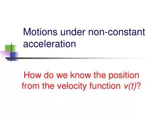
1. Motions under non-constant acceleration How do we know the position from the velocity function v(t)?

2. Displacement from a Velocity - Time Graph • The displacement of a particle during the time interval ti to tf is equal to the area under the curve between the initial and final points on a velocity-time curve

3. Displacement during a time interval • First, we divide the time range from Ta to Tf into N equal intervals • Displacement Dxn during the n-th interval

4. Total displacement from Ta to Tf In the limit as N approaches to infinite, the time interval Dt becomes smaller and smaller. Displacement is the area under the curve of v(t).

5. Position xf at Tf with initial position xa at Ta If the function v(t) is constant in time,

6. How do we know the velocity from the acceleration function a(t) ?

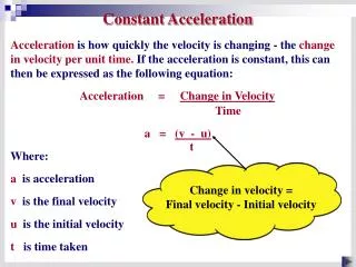
7. Velocity vf at Tf with initial velocity va at Ta If the function a(t) is constant in time,

8. Position xf at Tf under a constant acceleration with initial velocity va at Ta=0

9. Chapter 3 Motion in Two Dimensions

10. 3.1 Position and Displacement • The position of an object is described by its position vector, • The displacement of the object is defined as the change in its position Fig 3.1

11. Average Velocity • The average velocity is the ratio of the displacement to the time interval for the displacement • The direction of the average velocity is the direction of the displacement vector, Fig 3.2

12. Average Velocity, cont • The average velocity between points is independent of the path taken • This is because it is dependent on the displacement, which is also independent of the path • If a particle starts its motion at some point and returns to this point via any path, its average velocity is zero for this trip since its displacement is zero

13. Instantaneous Velocity • The instantaneous velocity is the limit of the average velocity as ∆t approaches zero

14. Instantaneous Velocity, cont • The direction of the instantaneous velocity vector at any point in a particle’s path is along a line tangent to the path at that point and in the direction of motion • The magnitude of the instantaneous velocity vector is the speed

15. Average Acceleration • The average acceleration of a particle as it moves is defined as the change in the instantaneous velocity vector divided by the time interval during which that change occurs.

16. Average Acceleration, cont • As a particle moves, can be found in different ways • The average acceleration is a vector quantity directed along Fig 3.3

17. Instantaneous Acceleration • The instantaneous acceleration is the limit of the average acceleration as approaches zero

18. Producing An Acceleration • Various changes in a particle’s motion may produce an acceleration • The magnitude of the velocity vector may change • The direction of the velocity vector may change • Even if the magnitude remains constant • Both may change simultaneously

19. 3.2 Kinematic Equations for Two-Dimensional Motion • When the two-dimensional motion has a constant acceleration, a series of equations can be developed that describe the motion • These equations will be a generlization of those of one-dimensional kinematics to the vector form.

20. Kinematic Equations, 2 • Position vector • Velocity • Since acceleration is constant, we can also find an expression for the velocity as a function of time:

21. Kinematic Equations, 3 • The velocity vector can be represented by its components • is generally not along the direction of either or Fig 3.4(a)

22. Kinematic Equations, 4 • The position vector can also be expressed as a function of time: • This indicates that the position vector is the sum of three other vectors: • The initial position vector • Thedisplacement resulting from • The displacement resulting from

23. Kinematic Equations, 5 • The vector representation of the position vector • is generally not in the same direction as or as • and are generally not in the same direction Fig 3.4(b)

24. Kinematic Equations, Components • The equations for final velocity and final position are vector equations, therefore they may also be written in component form • This shows that two-dimensional motion at constant acceleration is equivalent to two independent motions • One motion in the x-direction and the other in the y-direction

25. Kinematic Equations, Component Equations • becomes • vxf = vxi + axt and • vyf = vyi + ayt • becomes • xf = xi + vxit + 1/2 axt2 and • yf = yi + vyit + 1/2 ayt2

31. 3.3 Projectile Motion • The motion of an object under the influence of gravity only • The form of two-dimensional motion

32. Assumptions of Projectile Motion • The free-fall acceleration is constant over the range of motion • And is directed downward • The effect of air friction is negligible • With these assumptions, the motion of the object will follow

33. Projectile Motion Vectors • The final position is the vector sum of the initial position, the displacement resulting from the initial velocity and that resulting from the acceleration • This path of the object is called the trajectory Fig 3.6

34. Analyzing Projectile Motion • Consider the motion as the superposition of the motions in the x- and y-directions • Constant-velocity motion in the x direction • ax = 0 • A free-fall motion in the y direction • ay = -g

35. Verifying the Parabolic Trajectory • Reference frame chosen • y is vertical with upward positive • Acceleration components • ay = -g and ax = 0 • Initial velocity components • vxi = vi cos qi and vyi = vi sin qi

36. Projectile Motion – Velocity at any instant • The velocity components for the projectile at any time t are: • vxf = vxi = vi cos qi = constant • vyf = vyi – g t = vi sin qi – g t

37. Projectile Motion – Position • Displacements • xf = vxit = (vi cos qi)t • yf = vyit + 1/2ay t2 = (vi sinqi)t - 1/2 gt2 • Combining the equations gives: • This is in the form of y = ax – bx2 which is the standard form of a parabola

38. What are the range and the maximum height of a projectile • The range, R, is the maximum horizontal distance of the projectile • The maximum height, h, is the vertical distance above the initial position that the projectile can reaches. Fig 3.7

39. Projectile Motion Diagram Fig 3.5

40. Projectile Motion – Implications • The y-component of the velocity is zero at the maximum height of the trajectory • The accleration stays the same throughout the trajectory

41. Height of a Projectile, equation • The maximum height of the projectile can be found in terms of the initial velocity vector: • The time to reach the maximum:

42. Range of a Projectile, equation • The range of a projectile can be expressed in terms of the initial velocity vector: • The time of flight = 2tm • This is valid only for symmetric trajectory

43. More About the Range of a Projectile

44. Range of a Projectile, final • The maximum range occurs at qi = 45o • Complementary angles will produce the same range • The maximum height will be different for the two angles • The times of the flight will be different for the two angles

45. Non-Symmetric Projectile Motion