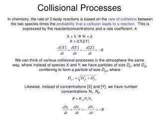
Collisional Processes
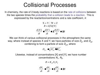
Collisional Processes. In chemistry, the rate of 2-body reactions is based on the rate of collisions between the two species times the probability that a collision leads to a reaction. This is expressed by the reactantconcentrations and a rate coefficient, k :. X + Y W + Z

Collisional Processes
E N D
Presentation Transcript
Collisional Processes In chemistry, the rate of 2-body reactions is based on the rate of collisions between the two species times the probability that a collision leads to a reaction. This is expressed by the reactantconcentrations and a rate coefficient, k: X + Y W + Z R = k[X][Y] We can think of various collisional processes in the atmosphere the same way, where instead of species X and Y, we have particles of size Dp1 and Dp2 combining to form a particle of size Dp3, where Likewise, instead of concentrations [X] and [Y], we have number concentrations N1, N2. R = K12N1N2
Review of Coagulation • Coagulation by diffusion: • Collision rate depends on the particles’ diffusivities, D1 and D2. • Important for aerosol smaller than 1 mm. • Main sink for the Aitken/nucleation modes of aerosols • Main source for the Accumulation mode • Di usually includes the slip correction factor, since Dpiis generally small • b is a kinetic correction that is important for Dpi < 100 nm. • You usually use tables (13.2, 13.3, Fig 13.5) for K12. Some particles bounce instead of sticking on collision. If the probability of the particles “sticking” on collision a < 1, use S+P Equation (13.56) to calculate K and b. Useful formulae: “self-coagulation” For Kn << 1 (i.e. Dpi >> 100 nm)
Shear Coagulation • Coagulation by laminar shear: • Collision rate depends on airflow shear • Important for aerosol and cloud drops larger than 100 nm. • Usually relevant in laboratory conditions • The basic concept between turbulent coagulation, relevant in atmosphere (discussed later) • Ignores kinetic effects + sticking probability – basically an overestimate
Shear Coagulation • Coagulation by turbulent shear: • Collision rate depends on turbulent kinetic energy density, ek. • Important for cloud drops (generally > 5 mm). • Same concept as laminar shear – uses turbulent theory to estimate typical shear near a droplet in a turbulent field • Purely theoretical – ignores a number of effects, including inertial motion of particles, flow-following behavior of smaller drops, sticking probability, etc.
Gravitational Settling • Coagulation by gravitational settling: • Collision rate depends on differential terminal velocities, vt,i. • Important for drizzle and rain drops (generally > 100 mm). • Depends on collision volume and a collision efficiency, E • Usually, Dp1 = drizzle drop (> 100 mm), Dp2 = cloud drop (< 100 mm) • For drizzle drops, find terminal velocity from • S+P Section 9.3 using Figure 9.7 –OR- • S+P Eqs. 9.32 and 9.44 (less accurate) • E is the combination of • The probability of a collision due to bending of the trajectories • The probability of coalescence due to bounceoff
Collision Efficiency Et=total collection efficiency E = Collision efficiency Ec = Coalescence probability For a very detailed empirical formulation of E (hence y), see the discussion surrounding S+P Eq. 20.53. Otherwise, simply use S+P figure 17.29
The Big Picture Convolve this picture (for 1 mm particles only) with the concentration of the other particle sizes to estimate the collisional lifetime of the drop. Note that collisions with smaller particles will only incrementally affect the size of the 1 mm target. Note that shear never dominates – it can be a correction, though. Why does Brownian motion have have that dip in the middle? Why does sedimentation have a much stronger dip in the middle?