Implementing the MAR-1 Algorithm
Implementing the MAR-1 Algorithm. A conceptual walkthrough. Steps for Implementing MAR-1 models. Ecological decisions Data formatting Data transformations Model selection Estimated MAR-1 parameter given model Model fit metrics, model fit diagnostics Stability properties

Implementing the MAR-1 Algorithm
E N D
Presentation Transcript
Implementing the MAR-1 Algorithm A conceptual walkthrough
Steps for Implementing MAR-1 models • Ecological decisions • Data formatting • Data transformations • Model selection • Estimated MAR-1 parameter given model • Model fit metrics, model fit diagnostics • Stability properties • Bootstrap confidence intervals
Step 1: Make ecological decisions • What interactions are you interested in? • Do you have enough data?
Step 1: Make ecological decisions • Are you missing major players in your community? Birds Insects Plants
Step 1: Make ecological decisions • Make apriori decisions to simplify the foodweb based on ecological knowledge about the system. VariateCovariate
Step 1: Make ecological decisions • What are the important abiotic covariates? rainfall temperature hunting pressure date years since last fire rabies prevalence storm frequency road density
Step 1: Complex system reduced to a smaller set of variates and covariates to address the interactions of interest
Step 2: Format the data • No missing values • One column for each variate and covariate • One row for each time step
Step 3: Transform the data • Counts for species should be transformed by the natural logarithm. LN
Step 3: Transform the data • You may need to transform by z-scores also if the data are on very different scales. LN Z
Step 3: Specify the relationship between the co-variates and the rates of growth The relationship for biotic covariates is system specific Spp covariates would be ln transformed to be consistent with the MAR framework
Step 3: Transform the co-variates • The transformation for the abiotic covariates is determined by the relationship between covariates and spp growth rates. The best transformation is not necessarily a natural logarithm. ?
Step 4: Choose the Model Selection Method • Compare a specified set of candidate models • testing a set of particular hypotheses • want to use a restricted set of prior models (over which the best is picked or over which models are averaged).
Step 4: Choose the Model Selection Method • Compare a specified set of candidate models • testing a set of particular hypotheses • want to use a restricted set of prior models (over which the best is picked or over which models are averaged). • Search over the set of all possible models • constrain models by known interactions • rank models by a model selection metric (such as AIC or BIC) • select the best fit model or use a model average
Step 4: Choose a model comparison approach • Compare a specified set of candidate models Hawks Foxes Lizards Snakes Rainfall Mice Insects 1 0 1 1 0 1 0 Hawks Hawks Foxes 0 1 0 0 Foxes 0 1 0 Lizards 0 0 1 0 Lizards 1 0 1 Sparse model Snakes 1 0 0 1 Snakes 1 1 0 Hawks Foxes Lizards Snakes Rainfall Mice Insects 1 0 1 1 0 1 0 Hawks Hawks Foxes 0 1 1 1 Foxes 0 1 0 Full model Lizards 1 1 1 1 Lizards 1 0 1 Snakes 1 1 1 1 Snakes 1 1 0
Step 4: Choose a model comparison approach • Search over all models and choose the best
Hawks Foxes Lizards Snakes Rainfall Mice Insects 1 0 1 1 0 1 0 Hawks Hawks Foxes 0 1 1 1 Foxes 0 1 0 Lizards 1 1 1 1 Lizards 1 0 1 Snakes 1 1 1 1 Snakes 1 1 0 Step 4: Choose a model comparison approach A. Begin with a proposed model (randomly selected) 1 = included interaction 0 = excluded interaction
Hawks Foxes Lizards Snakes Rainfall Mice Insects 0.25 0 0.22 0.09 0 0.11 -0.15 Hawks Hawks Foxes 0 0.79 0 0 Foxes 0 0.21 0 Lizards 0 0 0.55 0 Lizards 0.11 0 0.55 Snakes -0.51 0 0 0.61 Snakes 0.05 0.05 0.27 Step 5: Iterate through the possible models (CLS method) A. Begin with a proposed model (randomly selected) B.Perform a CLS regression on the proposed model to get values for the included interactions
Step 5: Iterate through the possible models (CLS method) A. Begin with a proposed model (randomly selected) B. Perform a CLS regression on the proposed model to get values for the included interactions C. Use this model to compute the Akaike or Bayesian Information Criterion for that model (AIC or BIC)
Hawks Hawks Foxes Foxes Lizards Lizards Snakes Snakes Rainfall Rainfall Mice Mice Insects Insects 1 1 0 0 1 1 1 1 0 0 1 1 1 1 Hawks Hawks Hawks Hawks Foxes Foxes 0 0 1 1 0 0 0 0 Foxes Foxes 0 0 1 1 0 0 Lizards Lizards 0 0 0 1 1 1 0 0 Lizards Lizards 1 1 0 0 1 1 Snakes Snakes 1 1 0 0 0 0 1 1 Snakes Snakes 1 1 1 1 1 1 Step 5: Iterate through the possible models (CLS method) D. Randomly change one matrix element to its opposite
Step 5: Iterate through the possible models (CLS method) D. Randomly change one matrix element to its opposite E. Re-run the CLS regression, find the AIC or BIC, and compare
Step 5: Iterate through the possible models (CLS method) D. Randomly change one matrix element to its opposite E. Re-run the CLS regression, find the AIC or BIC, and compare G. If the new model has a lower AIC/BIC, keep it. Otherwise, keep the old one.
Step 5: Iterate through the possible models (CLS method) D. Randomly change one matrix element to its opposite E. Re-run the CLS regression, find the AIC or BIC, and compare G. If the new model has a lower AIC/BIC, keep it. Otherwise, keep the old one. H. Repeat hundreds of times, until you have the model that generates the lowest possible AIC
Hawks Foxes Lizards Snakes Rainfall Mice Insects 0.89 0 0.27 0 0 0.54 -0.11 Hawks Hawks Foxes 0 0.54 0 0 Foxes 0 0.21 0 Lizards 0 0 0.15 -0.28 Lizards 0.11 0 0.56 Snakes -0.51 0 0.14 0.39 Snakes -0.04 0.15 0.18 Step 5: Iterate through the possible models (CLS method) • The search procedure finds the model that best explains the data with the lowest AIC or BIC
Step 6: Compute stability properties Once you know the interaction matrix, and the covariance matrix, you can compute the stability properties of the stationary distribution X
Step 6: Compute stability properties • Variance of the stationary distribution • eigenvalues • det(B)2/p
Step 6: Compute stability properties • Variance of the stationary distribution • eigenvalues • det(B)2/p • Return time to the stationary distribution • max(lB) • max(lBB)
Step 6: Compute stability properties • Variance of the stationary distribution • eigenvalues • det(B)2/p • Return time to the stationary distribution • max(lB) • max(lBB) • Reactivity of the stationary distribution • max(lBB)-1 • -tr(S)/tr(V)
Step 7: Bootstrap re-sampling • To obtain CIs on the parameter estimates, one can perform bootstrap re-sampling.
Step 7: Bootstrap re-sampling • To obtain CIs on the parameter estimates, one can perform bootstrap re-sampling • Basically, you scramble up the Et matrices • To create a bootstrapped E time series • From which you create a bootstrapped X time series Xt = A + BXt -1 + CUt-1 + Et
Step 7: Bootstrap re-sampling • To obtain CIs on the parameter estimates, one can perform bootstrap re-sampling • Repeat thousands of times to create thousands of bootstrapped data sets • From each bootstrapped data set, one re-estimates the A, B, and C matrices to get bootstrapped confidence intervals Xt = A + BXt -1 + CUt-1 + Et
Step 7: Bootstrap estimates example Means with 95% CI ranges (made up example) Hawks Foxes Lizards Snakes Hawks 0.25 (0.20,0.30) 0.05 (0.01, 0.09) 0.22 (0.16, 0.28) 0.09 (0.07, 0.11) Foxes 0 0.79 (0.59, 0.99) 0 0 Lizards 0.07 (-0.03, 0.17) 0 0.55 (0.43, 0.67) 0 Snakes -0.51 (-0.62, -0.40) 0 0 0.61 (0.54, 0.68) • Can obtain CIs on A and C matrices and on all the stability metrics also in the same way.
Data Transformations Type of model selection Manually specify model Search over all model possibilities Estimate A, B, & C matrices Estimate stability metrics, model fit diagnostics, and model selection metrics Bootstrap to obtain bootstrapped CIs Use simulation to test robustness of assumptions
That’s a lot of work. It would be nice if there was a computer program that could do it all for you….
That’s a lot of work. It would be nice if there was a computer program that could do it all for you…. There is! (We will show it to you after lunch and use it in the hands-on section.)