Download

1 / 25
250 likes | 499 Views
Chapter Outline 13.1 Introduction Box 13.1 A Survey of Spatial Interpolation among GIS Packages 13.2 Elements of Spatial Interpolation 13.2.1 Control Points 13.2.2 Type of Spatial Interpolation 13.3 Global Methods 13.3.1 Trend Surface Analysis

E N D
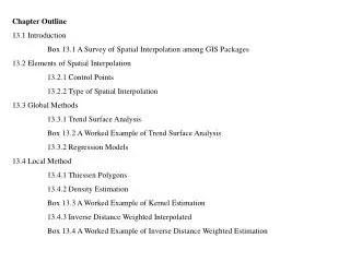
Chapter Outline 13.1 Introduction Box 13.1 A Survey of Spatial Interpolation among GIS Packages 13.2 Elements of Spatial Interpolation 13.2.1 Control Points 13.2.2 Type of Spatial Interpolation 13.3 Global Methods 13.3.1 Trend Surface Analysis Box 13.2 A Worked Example of Trend Surface Analysis 13.3.2 Regression Models 13.4 Local Method 13.4.1 Thiessen Polygons 13.4.2 Density Estimation Box 13.3 A Worked Example of Kernel Estimation 13.4.3 Inverse Distance Weighted Interpolated Box 13.4 A Worked Example of Inverse Distance Weighted Estimation
13.4.4 Thin-plate Splines Box 13.5 Radial Basis Functions Box 13.6 A Worked Example of Thin-plate Splines with Tension 13.4.5 Kriging 13.4.5.1 Ordinary Kriging Box 13.7 A Worked Example of Ordinary Kriging Estimation 13.4.5.2 Universal Kriging Box 13.8 A Worked Example of Universal Kriging Estimation 13.4.5.3 Other Kriging Methods 13.5 Comparison of Spatial Interpolation Methods Box 13.9 Spatial Interpolation using ArcGIS
Applications: Spatial Interpolation Task 1: Use Trend Surface Analysis for Global Interpolation Task 2: Use Kernel Density Estimation for Local Interpolation Task 3: Use IDW for Local Interpolation Task 4: Compare Two Splines Methods Task 5: Use Ordinary Kriging for Local Interpolation Task 6: Use Universal Kriging for Local Interpolation Task 7: Use Cokriging for Local Interpolation
A map of 105 weather stations in Idaho and their 30-year average annual precipitation values
The unknown value at Point 0 is interpolated by five surrounding stations with known values.
An isoline map of a third-order trend surface created from 105 control points with annual precipitation values.
(a) (b) (c) Three search methods for sample points: (a) find the closest points to the point to be estimated, (b) find points within a radius, and (c) find points within each of the four quadrants.
The diagram shows known points, Delaunay triangulation in thinner lines, and Thiessen polygons in thicker lines.
The simple density estimation method is used to compute the number of deer sightings per hectare from the point data.
Kernel k() Bandwidth A kernel function, which represents a probability density function, looks like a “bump” above a grid.
The kernel estimation method is used to compute the number of sightings per hectare from the point data. The letter X marks the cell, which is used as an example in Box 13.3.
An annual precipitation surface map created by the inverse distance weighted method
An isohyet map created by the inverse distance weighted method
Semivariance Sill Nuggett Distance Range Actual Variance Predicted Variance A semivariogram shows semivariances along the y-axis and distances along the x-axis.
Five mathematical models for fitting semivariograms: Gaussian, linear, spherical, circular, and exponential
An isohyet map created by ordinary kriging with the linear model
The map shows the standard deviation of the annual precipitation surface created by ordinary kriging with the linear model.
A semivariogram constructed from annual precipitation values at 105 weather stations in Idaho. The linear model provides the trend line.
An isohyet map created by universal kriging with the linear drift
The map shows the standard deviation of the annual precipitation surface created by universal kriging with the linear drift.
The map shows the difference between surfaces generated from the regularized splines method and the inverse distance squared method. A local operation, in which one surface grid was subtracted from the other, created the map.
The map shows the difference between surfaces generated from the ordinary kriging with linear model method and the regularized splines method.
PRISM, Natural Resources Conservation Service (NRCS) http://www.ftw.nrcs.usda.gov/prism/prismdata.html/