Download
1 / 55
560 likes | 800 Views
EE534 VLSI Design System Summer 2004 Lecture 05: Resistance and Static CMOS inverter. CMOS Inverter: Dynamic. Transient, or dynamic , response determines the maximum speed at which a device can be operated. V DD. Last lecture’s focus. V out = 0. C L. t pHL = f(R n , C L ). R n.

E N D
EE534VLSI Design SystemSummer 2004 Lecture 05: Resistance and Static CMOS inverter
CMOS Inverter: Dynamic • Transient, or dynamic, response determines the maximum speed at which a device can be operated. VDD Last lecture’s focus Vout = 0 CL tpHL = f(Rn, CL) Rn Vin = V DD Today’s focus
CDB2 CDB1 Review: Sources of Capacitance Vout Vin Vout2 CL CG4 M2 M4 CGD12 Vout Vout2 Vin Cw M3 M1 CG3 intrinsic MOS transistor capacitances extrinsic MOS transistor (fanout) capacitances wiring (interconnect) capacitance
Sources of Resistance • MOS structure resistance - Ron • Source and drain resistance • Contact (via) resistance • Wiring resistance Top view Poly Gate Drain n+ Source n+ W L
VGS VT Ron D S MOS Structure Resistance • The simplest model assumes the transistor is a switch with an infinite “off” resistance and a finite “on” resistance Ron • However Ron is nonlinear, so use instead the average value of the resistances, Req, at the end-points of the transition (VDD and VDD/2) Req = ½ (Ron(t1) + Ron(t2)) Req = ¾ VDD/IDSAT (1 – 5/6 VDD)
x105 (for VGS = VDD, VDS = VDDVDD/2) Req (Ohm) VDD (V) Equivalent MOS Structure Resistance • The on resistance is inversely proportional to W/L. Doubling W halves Req • For VDD>>VT+VDSAT/2, Req is independent of VDD (see plot). Only a minor improvement in Req occurs when VDD is increased (due to channel length modulation) • Once the supply voltage approaches VT, Req increases dramatically Req (for W/L = 1), for larger devices divide Req by W/L
Source and Drain Resistance G • More pronounced with scaling since junctions are shallower • With silicidation Ris reduced to the range 1 to 4 / D S RS RD RS,D = (LS,D/W)R where LS,D is the length of the source or drain diffusion R is the sheet resistance of the source or drain diffusion (20 to 100 /)
Contact Resistance • Transitions between routing layers (contacts through via’s) add extra resistance to a wire • keep signals wires on a single layer whenever possible • avoid excess contacts • reduce contact resistance by making vias larger (beware of current crowding that puts a practical limit on the size of vias) or by using multiple minimum-size vias to make the contact • Typical contact resistances, RC, (minimum-size) • 5 to 20 for metal or poly to n+, p+ diffusion and metal to poly • 1 to 5 for metal to metal contacts • More pronounced with scaling since contact openings are smaller
Wire Resistance L L R = = A H W Sheet Resistance R L R1 = R2 H = W
Skin Effect • At high frequency, currents tend to flow primarily on the surface of a conductor with the current density falling off exponentially with depth into the wire W • = (/(f)) where f is frequency = 4 x 10⁻⁷ H/m so the overall cross section is ~ 2(W+H) • = 2.6 m for Al at 1 GHz H • The onset of skin effect is at fs - where the skin depth is equal to half the largest dimension of the wire. fs = 4 / ( (max(W,H))2) • An issue for high frequency, wide (tall) wires (i.e., clocks!)
Skin Effect for Different W’s for H = .70 um 1E8 1E9 1E10 • A 30% increase in resistance is observe for 20 m Al wires at 1 GHz (versus only a 1% increase for 1 m wires)
The Wire transmitters receivers schematic physical
Wire Models • Interconnect parasitics (capacitance, resistance, and inductance) • reduce reliability • affect performance and power consumption All-inclusive (C,R,l) model Capacitance-only
Parasitic Simplifications • Inductive effects can be ignored • if the resistance of the wire is substantial enough (as is the case for long Al wires with small cross section) • if the rise and fall times of the applied signals are slow enough • When the wire is short, or the cross-section is large, or the interconnect material has low resistivity, a capacitance only model can be used • When the separation between neighboring wires is large, or when the wires run together for only a short distance, interwire capacitance can be ignored and all the parasitic capacitance can be modeled as capacitance to ground
Simulated Wire Delays L Vin Vout L/10 L/4 L/2 L voltage (V0) time (nsec)
silicide polysilicon SiO2 + + n n p Overcoming Interconnect Resistance • Selective technology scaling • scale W while holding H constant • Use better interconnect materials • lower resistivity materials like copper • As processes shrink, wires get shorter (reducing C) but they get closer together (increasing C) and narrower (increasing R). So RC wire delay increases and capacitive coupling gets worse. • Copper has about 40% lower resistivity than aluminum, so copper wires can be thinner (reducing C) without increasing R • use silicides (WSi2, TiSi2, PtSi2 and TaSi) • Conductivity is 8-10 times better than poly alone • Use more interconnect layers • reduces the average wire length L (but beware of extra contacts)
IBM CMOS-8S CU, 0.18m - 0.10 M7 - 0.10 M6 - 0.50 M5 - 0.50 M4 - 0.50 M3 - 0.70 M2 - 0.97 M1 Wire Spacing Comparisons Intel P858 Al, 0.18m Intel P856.5 Al, 0.25m - 0.07 M6 - 0.05 M5 - 0.08 M5 - 0.12 M4 - 0.17 M4 - 0.33 M3 - 0.49 M3 - 0.33 M2 - 0.49 M2 - 1.11 M1 - 1.00 M1 Scale: 2,160 nm From MPR, 2000
SYSTEM + G MODULE S D n+ n+ GATE CIRCUIT CIRCUIT Vin Vin Vout Vout DEVICE Design Abstraction Levels
CMOS:the most abundant devices on earth • At present, complementary MOS or CMOS has replaced NMOS at all level of integration, in both analog and digital applications. • The basic reason of this replacement is that the power dissipation in CMOS logic circuits is much less than in NMOS circuits, which makes CMOS very attractive. • Although the processing is more complicated for CMOS circuits than for NMOS circuits. • However, the advantages of CMOS digital circuits over NMOS circuits justify their use.
Simplified cross section of a CMOS inverter • In the fabrication process, a separate p-well region is formed within the starting n-substrate. • The n-channel MOSFET is fabricated in the p-well region and p-channel MOSFET is fabricated in the n-substrate.
CL CMOS Inverter: A First Look VDD Vin Vout
CMOS Properties • Full rail-to-rail swing high noise margins • Logic levels not dependent upon the relative device sizes transistors can be minimum size ratioless • Always a path to Vdd or GND in steady state low output impedance (output resistance in k range) large fan-out (albeit with degraded performance) • Extremely high input resistance (gate of MOS transistor is near perfect insulator) nearly zero steady-state input current • No direct path steady-state between power and ground no static power dissipation • Propagation delay function of load capacitance and resistance of transistors
7 DC analysis of the CMOS inverter • The figure shows series combination of a CMOS inverter. • To form the input, gate of the two MOSFET are connected. • To form the output, the drains are connected together. • VI Vo • 1 0 • 0 1 VGS,n = Vin VDS,n = Vout The transistor KN is also known as “pull down” Device, it is pulling the output voltage down towards ground. The transistor KPis known as the “pull up” device because it is pulling the output voltage up towards VDD. This property speed up the operation considerably. Vou t= VOH = VDD Vout = VOL = 0 It is to be noted that the static power dissipation during both extreme cases (logic 1 or 0) is almost zero because iDp=iDn=0.
Review: Short Channel I-V Plot (NMOS) X 10-4 VGS = 2.5V VGS = 2.0V ID (A) VGS = 1.5V Linear dependence VGS = 1.0V VDS (V) NMOS transistor, 0.25um, Ld = 0.25um, W/L = 1.5, VDD = 2.5V, VT = 0.4V
Review: Short Channel I-V Plot (PMOS) • All polarities of all voltages and currents are reversed VDS (V) VGS = -1.0V VGS = -1.5V ID (A) VGS = -2.0V VGS = -2.5V X 10-4 PMOS transistor, 0.25um, Ld = 0.25um, W/L = 1.5, VDD = 2.5V, VT = -0.4V
VDD Vout CL CMOS Inverter VTC NMOS off PMOS res NMOS sat PMOS res NMOS sat PMOS sat Vout (V) NMOS res PMOS sat NMOS res PMOS off Vin (V)
NMOS in sat PMOS in non sat NMOS off PMOS in non sat NMOS in sat PMOS in sat NMOS in non sat PMOS in sat NMOS in nonsat PMOS off Complete voltage transfer characteristics, CMOS inverter
CMOS Inverter: VTC PMOS NMOS Vin=4V VCC Vin=3V Drain current IDS Vout Vin=2V Vin=1V Vin Vout = VDS VCC 0 1 2 3 4 • Output goes completely to Vcc and Gnd • Sharp transition region
VDD VDD Rp Vout Vout CL CL Rn Vin = 0 Vin = V DD CMOS Inverter: Switch Model of Dynamic Behavior • Gate response time is determined by the time to charge CL through Rp (discharge CL through Rn)
CMOS inverter operation Vcc • NMOS transistor: • Cutoff if Vin < VTN • Linear if Vout < Vin – VTN • Saturated if Vout > Vin – VTN • PMOS transistor • Cutoff if (Vin-VCC) < VTP → Vin < Vcc+VTP • Linear if (Vout-VCC)>Vin-Vcc-VTP → Vout>Vin - VTP • Sat. if (Vout-VCC)<Vin-Vcc-VTP → Vout < Vin-VTP Vin Vout
CMOS inverter design consideration • The CMOS inverter usually design to have, (i) VTN =|VTP| (ii) K´n(W/L)=K´p(W/L) But K´n>K´p (because n>p) How equation (ii) can be satisfied? This can be achieved if width of the PMOS is made two or three times than that of the NMOS device. This is very important in order to provide a symmetrical VTC, results in wide noise margin.
CMOS inverter design consideration (cont.) • Increase W of PMOS kp increases VTC moves to right kp=kn VCC • Increase W of NMOS kn increases VTC moves to left kp=5kn Vout kp=0.2kn • For VTH = Vcc/2 kn = kp Wn 2Wp VCC Vin
Good PMOS Bad NMOS Nominal Bad PMOS Good NMOS Impact of Process Variation on VTC Curve Vout (V) Vin (V) • Process variations (mostly) cause a shift in the switching threshold
Effects of Vth adjustment • Result from changing kp/kn ratio: • Inverter threshold VTH Vcc/2 • Rise and fall delays unequal • Noise margins not equal • Reasons for changing inverter threshold • Want a faster delay for one type of transition (rise/fall) • Remove noise from input signal: increase one noise margin at expense of the other
Concept of Noise Margins VI NML=VIL-VOL(noise margin for low input) NMH=VOH-VIH(noise margin for high input)
CMOS inverter: VIL • KCL: • Differentiate and set dVout/dVin to –1 • Solve simultaneously with KCL to find VIL