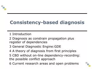
Consistency-based diagnosis
Consistency-based diagnosis. 1 Introduction 2 Diagnosis as constrain propagation plus register of dependencies 3 General Diagnostic En g ine:GDE 4 A theory of diagnosis from first principles 5 CBD without on-line dependency-recording: the possible conflict approach

Consistency-based diagnosis
E N D
Presentation Transcript
Consistency-based diagnosis 1 Introduction 2 Diagnosis as constrain propagation plus register of dependencies 3 General Diagnostic Engine:GDE 4 A theory of diagnosis from first principles 5 CBD without on-line dependency-recording: the possible conflict approach 6 Current research areas and open problems
Model-based Reasoning process oriented component oriented causal models process models structural models functional models behavioural models teleological models (similar to comp. oriented.) ... ... ... crisp probabilistic correct behaviour fault models .… extensional intensional .… time- varying quantitative qualitative static dynamic hierarchical flat discrete state change landmarks orders of magnitude ... derivatives intervals Automated Diagnosis Introduction Machine Learning Case-Based Reasoning Knowledge-Based Sytems Devices Software… Processes Medicine Application fields
Model-based diagnosis approaches • Control Theory / Engineering (FDI community) • Robuts Fault Detection and Isolation • (Global) Analytical Models, mainly • Generation and Analysis of Residuals (discrepancy) • Most commonly used techniques • State-observers • Parity-equations (Analytical Redundancy Relations) • Parameter Identification (or Estimation) • Artificial Inteligence (DX community) • Fault Isolation and Identification • (assumption: robust fault detection is available) • Qualitative Models (causal, constraints, semi-qualitative, etc.) • Conflict detection and candidate (diagnosis) generation • Diagnosis based on structure and behaviour • Consistency-based diagnosis • Abductive diagnosis • Consistency-based Diagnosis with fault models • BRIDGE (integration of DX and FDI) GDE
Consistency Based DiagnosisIntroduction Historical background • Second generation Expert Systems (Davis, 1982-84) • First works in USA, late 70s – early 80s (@ MIT, Stanford Univ.) • Solid theoretical theory (Reiter, 1987) • Early results: • mid/late-80s: static systems • late 80s, early 90s: dynamic systems • late 90s (mature) large systems GDE
Model-based diagnosis fundamental Behaviour Model Real System Diagnosis Predicted Behaviour Observed Behaviour Discrepancy (symptom) GDE
Consistency Based DiagnosisIntroduction • Main Model Based Diagnosis framework from DX community • Component oriented (ontology) • May be extended to processes / constraints • Knowledge: • structural + behavioural (local) models • models of components • Only models of correct behaviour GDE
Basic Assumptions (de Kleer 03) • Physical system • Set of interconnected components • Known desired function • Design achieves function • System is correct instance of design • All malfunctions caused by faulty component(s) • Behavioural information • Only indirect evidence GDE
Behavioural information: Behavioural models • Components are in some physical condition • e.g. a wire • Different physical conditions result in different behaviours Condition 1 Condition 2 Condition 3 Behaviour 1 Behaviour 3 Behaviour 2 GDE
Behavioural information: Ruling out behaviours • We cannot verify the presence of behaviours, but we can falsify them • After observing • We cannot infer behaviour 2, but we can reject behaviour 1 GDE
Consistency Based Diagnosis Intuition • Search for the model that is “compliant” with the observations Behaviour Model Real System Diagnosis Predicted Behaviour Observed Behaviour Discrepancy GDE
General Diagnostic Engine • GDE, de Kleer and Williams, 87 • First model based computational system for multiple faults • Main computational paradigm • Still in use! • Still a reference to compare any model- based proposal on DX community GDE
A X F M1 A1 B C Y M2 D G A2 Z M3 E A classic expository example:the polybox (de Kleer 87, 03) GDE
Model based approach to diagnosis Textbooks, design, first principles Model Real System Predicted Behaviour Observed Behaviour Discrepancy Diagnosis GDE
A [3] B [2] C [2] D [3] E [3] Observed Behaviour X F F M1 A1 [10] Y M2 G A2 [12] Z M3 GDE
Model based approach to diagnosis Textbooks, design, first principles Model Real System Predicted Behaviour Observed Behaviour Discrepancy Diagnosis GDE
A [3] B [2] C X 6 [2] F M1 D A1 [3] E Y M2 [3] G A2 Z M3 Local propagation (I) GDE
A [3] B X 6 F [2] M1 C A1 [2] D 6 [3] Y M2 E G [3] A2 Z M3 Local propagation (II) GDE
A [3] B [2] X 6 F F C M1 [2] A1 12 D [3] 6 Y M2 E [3] G A2 Z M3 Local propagation (III) GDE
A [3] B [2] X 6 F F C M1 [2] A1 12 D [3] 6 Y M2 E [3] G A2 Z M3 6 Local propagation (IV) GDE
A [3] B [2] X 6 F F C M1 [2] A1 12 D [3] 6 Y M2 E [3] G A2 12 Z M3 6 Local propagation (V) GDE
A [3] B [2] X 6 F F C M1 [2] A1 12 D [3] 6 Y M2 E [3] G A2 12 Z M3 6 Predicted Behaviour GDE
Model based approach to diagnosis Textbooks, design, first principles Model Real System Predicted Behaviour Observed Behaviour Discrepancy Diagnosis GDE
A [3] X 6 12 F F M1 B A1 [10] [2] C 6 [2] Y D M2 12 [3] G A2 [12] Z E M3 [3] 6 Candidates • Detect Symptoms: F=12 and F=10 • Generate Candidates: {M1}, {A1}, {M2, S2}, {M2, M3} GDE
A [3] B [2] C [2] D [3] E [3] Diagnosis for the polybox X 4 12 F F M1 A1 [10] 6 Y M2 12 G A2 [12] Z M3 6 GDE
A [3] B [2] C [2] D [3] E [3] Diagnosis for the polybox X 6 12 F F M1 A1 [10] 6 Y M2 10 G A2 [12] Z M3 6 GDE
A [3] B [2] C [2] D [3] E [3] Diagnosis for the polybox X 6 12 F F M1 A1 [10] 4 Y M2 12 G A2 [12] Z M3 6 GDE
A [3] B [2] C [2] D [3] E [3] M3 Diagnosis for the polybox X 6 12 F F M1 A1 10 4 Y M2 12 G A2 [12] Z 8 GDE
How GDE works? • Detecting every SYMPTOM Prediction: propagating on every direction (even non causal!) • Identifying CONFLICTS • Generating CANDIDATES GDE
A [3] B [2] X 6 F F C M1 [2] A1 12 D [3] 6 Y M2 E [3] G A2 12 Z M3 6 Prediction - Requirements • Modeling Structure • Modeling component behaviour • Predict overall behaviour GDE
Modelling Structure - Requirements • Determine the structural elements and interconections • Which entities can be the origin of malfunction? • Which parts can be replaced? • Which variables can be observed? • Reflect aspects and levels of (diagnostic) reasoning about the device behaviour GDE
Component-Oriented Modelling: Components and Connections • Systems: components linked by connections via terminals • Components: Normally physical objects • Resistors, diodes, voltage sources, tanks, valves • Terminals: unique comunication link • Connections:ideal connections (but may be modelled as components) • No resistance wires, loadless pipes... • Possible faults: defect components, broken connection GDE
Modelling Behaviour -Requirements • Describe behaviour of the structural elements: Locality • Goal: detecting discrepancies • Consider aspecs like • Generality: which kind of devices are to be diagnosed? • Robustness: which type of failure are to be detected • Reflect the diagnostic reasonig process (e.g. simplifications) • Which kind of information is (easily) available (e. g. qualitative information) GDE
Local behaviour models • Constrains / relations among • Input/Output variables • Internal parameters • Various directions • No implicit reference to or implicit assumptions about context (existence or state of other components) • Locality • Necessary for diagnosis: different context because something is broken; otherwise implicit hypothesys must be revised • Reusability: model library, compositionality GDE
Local behaviour model - Example • Or-gate • Variables: in1, in2,out • Domain dom(in1)=dom(in2)=dom(out)={0,1} • Relation {{0,0,0}, {1,0,1}, {0,1,1}, {1,1,1}} dom(in1) dom(in2) dom(out) • Inferences • in1 = 1 out = 1 • in2 = 1 out = 1 • in1=0 in2=0 out = 1 • out=0 in1=0 in2=0 • out=1 in1=0 in2=1 • out=1 in2=0 in1=1 causal direction non causal direction GDE
A f B p1 p2 Behaviour model of a valve • Relation: f = k A • Implicit assumption: pump is on and ok • Relation: IF on(B) and ok(B) THEN f= k A • Implicit assumption: a pump exists and is connected as in the diagram • Better: f = k’ (p1 – p2) A • Principle: no function in structure GDE
A B F F C M1 A1 D M2 E G A2 M3 Abstract model • Domain for each variable, var dom(var) = {OK, BAD, ?} • Model for each correct component, C IF for all input-variables, vari of C, vari = OK THEN for each output-variable, varo of C, varo = OK • To avoid masking of faults by correct components IF there exists an input-variable, vari of C, vari = BAD THEN for each output-variable, varo of C, varo = BAD GDE
Prediction - Principles • Infer the behaviour of the entire device from • Observations • Component models • Structural description • Preserve dependencies on component models • Propagate the effects of local models along the interaction paths (connections) • Propagate not only in the causal direction GDE
A [3] B [2] C X 6 [2] F M1 D A1 [3] E Y M2 [3] G A2 Z M3 PropagationCausal direction (I) • [A]=3 [C]=2 X=6 (M1) GDE
A [3] B X 6 F [2] M1 C A1 [2] D 6 [3] Y M2 E G [3] A2 Z M3 PropagationCausal direction (II) • [B]=2 [D]=3 Y=6 (M2) GDE
A [3] B [2] X 6 F F C M1 [2] A1 12 D [3] 6 Y M2 E [3] G A2 Z M3 PropagationCausal direction (III) • X=6 Y=6 F=12 (A1) GDE
A [3] B [2] X 6 F F C M1 [2] A1 [10] D [3] 4 Y M2 E [3] G A2 Z M3 Propagation“Backward” direction (II) • [F]=10 X=6 Y=4 (A1) GDE
Candidate Generation • Detecting SYMPTOMS (DISCREPANCIES) • Identifying (minimal) CONFLICTS • Generating (minimal) CANDIDATES GDE
Symptoms Real System Model Predicted Behaviour Observed Behaviour Discrepancy Diagnosis • Symptoms are contradictions that indicate an inconsistency between observations and correct behaviour • But other potential sources of contradictions • Imprecise measurements • Bugs in the model • Bugs in propagation GDE
Symptoms Detection • Symptoms occurs as contradictory values for one variable • Predicted plus observed • Predicted following two different paths • Discrete Variables • Static x=val1 x=val2 val1 val2 • Dynamic x=(val1, t1) x=(val2, t2) val1 val2 (t1 t2) • Continuous Variables • Quantitatives (static): • Intervals: x=i1 x=i2 (i1 i2) • Values: x=val1 x=val2 val1 val2 • Relations: xval1 xval2 • Qualitatives: distance,distance >Threshold GDE
A [3] B [2] C [2] D [3] E [3] Some symptoms for the polybox (I) 12 X 6 F F M1 [10] A1 6 Y M2 G [12] A2 Z M3 GDE
A [3] B [2] C [2] D [3] E [3] Some symptoms for the polybox (II) X 6 F F M1 [10] A1 4 Y M2 6 G [12] A2 Z M3 GDE
A [3] B [2] C [2] D [3] E [3] Some symptoms for the polybox (III) X X X 6 6 F F F F M1 [10] A1 4 Y Y M2 M2 10 G G [12] A2 Z Z M3 6 6 GDE
A [3] B [2] C [2] D [3] E [3] Some symptoms for the polybox (IV) 6 X 12 F F M1 4 A1 [10] 6 Y M2 4 10 G A2 [12] 6 Z M3 8 GDE
Identify conflicts • Conflict (informal):set of correctness assumtions underlying discrepancies • Polybox (minimal) conflicts • F=[10] F=12 {M1, M2, A1}, {M1, M3, A1, A2} • X=6 X=4 {M1, M2, A1}, {M1, M3, A1, A2} • Y=6 Y=4 {M1, M2, A1}, {M1, M3, A1, A2} • Z=6 Z=8 {M1, M3, A1, A2} • G=[12] G=10 {M1, M3, A1, A2} • By definition,any superset of a conflic set is a conflict • {M1, M2, A1} {M1, M2, A1, A2} {M1,M2, M3, A1, A2} • Minimal conflict: conflict no proper subset of which is a conflict • It is essential to represent the conflicts through the set of minimal conflicts (to avoid combinatorial explosion) GDE
Conflicts latice [M1, M2, M3, A1, A2] [M1, M2, M3, A2] [M1, M3, A1, A2] [M2, M3, A1, A2] [M1, M2, A1, A2] [M1, M2, M3, A1] [ M3, A1, A2] [M1, M2, M3] [M1, M2, A1] [M1, M2, A2] [M1, M3, A1] [M1, M3, A2] [M2, M3 A1] [M1, A1, A2] [M2, M3, A2] [M2, A1, A2] [M1, M2] [M1, M3] [M1, A1] [M2, M3] [M1, A2] [M2, A1] [M2, A2] [ M3, A1] [ M3, A2] [ A1, A2] [M1] [M2] [M3] [A1] [A2] GDE [ ]