Download

1 / 20
200 likes | 327 Views
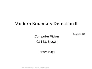
Modern Boundary Detection II. Szeliski 4.2. Computer Vision CS 143, Brown James Hays. Many slides Michael Maire , Jitendra Malek. Today’s lecture. pB boundary detector, from “local” to “global” Finding Junctions Sketch Tokens.

E N D
Modern Boundary Detection II Szeliski 4.2 Computer Vision CS 143, Brown James Hays Many slides Michael Maire, JitendraMalek
Today’s lecture • pB boundary detector, from “local” to “global” • Finding Junctions • Sketch Tokens
Sketch Tokens: A Learned Mid-levelRepresentation for Contour and Object Detection Joseph Lim, C Lawrence Zitnick, Piotr DollarCVPR 2013
Image Features – 21350 dimensions! • 35x35 patches centered at every pixel • 35x35 “channels” of many types: • Color (3 channels) • Gradients (3 unoriented + 8 oriented channels) • Sigma = 0, T heta = 0, pi/2, pi, 3pi/2 • Sigma = 1.5, Theta = 0, pi/2, pi, 3pi/2 • Sigma = 5 • Self Similarity • 5x5 maps of self similarity within the above channels for a particular anchor point.
Self-similarity features Self-similarity features: The L1 distance from the anchor cell (yellow box) to the other 5 x 5 cells are shown for color and gradient magnitude channels. The original patch is shown to the left.
Learning • Random Forest Classifiers, one for each sketch token + background, trained 1-vs-all • Advantages: • Fast at test time, especially for a non-linear classifier. • Don’t have to explicitly compute independent descriptors for every patch. Just look up what the decision tree wants to know at each branch.
Learning Frequency of example features being selected by the random forest: (first row) color channels, (second row) gradient magnitude channels, (third row) selected orientation channels.
Combining sketch token detections • Simply add the probability of all non-background sketch tokens • Free parameter: number of sketch tokens • k = 1 works poorly, k = 16 and above work OK.
Summary • Distinct from previous work, cluster the human annotations to discover the mid-level structures that you want to detect. • Train a classifier for every sketch token. • Is as accurate as any other method while being 200 times faster and using no global information.