Download
1 / 38
420 likes | 653 Views
Radiative Transitions between Electronic States. November 14, 2002. Michelle. Blackbody Radiation Wavelength dependence of energy distribution of light emitted by a hot object. Photoelectric Effect Wavelength dependence of energy of electrons emitted when light strikes a metal.

E N D
Radiative Transitions between Electronic States November 14, 2002. Michelle
Blackbody Radiation Wavelength dependence of energy distribution of light emitted by a hot object Photoelectric Effect Wavelength dependence of energy of electrons emitted when light strikes a metal From the perspective of absorption and emission it is more convenient to think of light in terms of an oscillating electromagnetic wave 4.1 “Paradigm” Shifts • Maxwell light as electromagnetic waves Planck Quantization of energy E = h Einstein Photons - quantized light consisting of particles possessing “bundles” of energy • DeBroglie light as a particle with wave properties • E = h = h(c/) = pc
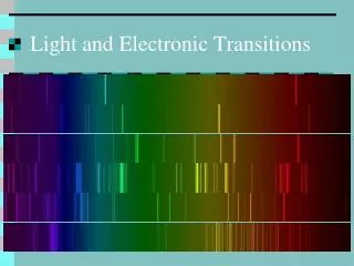
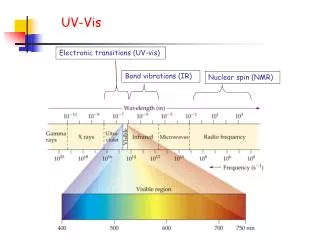
4.2-4.3 Absorption and Emission Transitions between electronic energy levels accompanied by absorption or emission of light Photochemical region of the spectrum: 200-700 nm 143 kcal mol-1-41 kcal mol-1 valence orbital (, , n) antibonding orbital (*, *) Chromophore: atom or group acting as a light absorber Lumophore: atom or group acting as a light emitter C=O C=C C=C-C=C C=C-C=O aromatics Molar absorptivity measures “absorption strength” units cm-1M-1NOT cm2mol-1
Dipoles as a model for interactions between electrons and light • oscillating electric dipole field of the electromagnetic wave • oscillating dipoles due to electrons moving in orbitals • Dipole-dipole interactions are through space and don’t require orbital overlap • (Interactions requiring overlap are “exchange interactions”) • Examples of dipolar interactions: London dispersion forces, EPR, NMR, large splittings for crystals (exciton interactions) 4.4 The Nature of Light The classical theory of light is a convenient starting point providing a pictorial and understandable physical representation of the interaction of light and molecules classical theory can be improved by applying quantum interpretations of basic concepts (orbital, quantized energy etc.) Exciton migration: electron-hole pair hopping from molecule to molecule in a crystal
4.4 Dispersion Forces Correlation of fluctuations in electronic charge distributions in molecules • Dipole on A drives formation of dipole on B and vice versa • Fluctuating dipoles are in “resonance” E ~ ABR-3AB True for all dipole-dipole interactions, magnetic or electric Energy of the dipole-dipole interaction falls off as A and B move apart, given by R-6AB
4.4 Light as an Oscillating Electric Field • Frequency () of oscillating field must “match” a possible electronic oscillation frequency (conservation of energy) • There must be an interaction or coupling between the field (oscillating dipoles) and the electron • Interaction strength depends on field dipole and induced dipole strength as well as distance between the two. • Laws of conservation of angular momentum must be obeyed (electrons, nuclei, spins) • Spin change is highly resisted in absorption due to time constraints *the most important interaction between the electromagnetic field and the electrons of a molecule can be modeled as the interaction of 2 oscillating dipole systems that behave as reciprocal energy-donor, energy-acceptors
electric field Direction of propogation H magnetic field 4.4 Light as an Oscillating Electric Field If the field can couple to the electrons it can exchange energy by driving the system into resonance at a frequency common to both A light wave generates a time-dependent force field F absorption: photons being removed from the electromagnetic field emission: photons being added (?) to the electromagnetic field ABSORPTION (reverse for emission)
4.4 Light as an Oscillating Electric Field • Radiative transitions between states are induced by perturbations which make the two states”look alike” by inducing a resonance • Resonance requires that the two states have the same energy and momentum characteristics and a common frequency for resonance E = h Energy difference between two states Frequency of light wave oscillation The energy of the photon must exactly match the the energy level difference in the molecule
F = e + e[H v] c 4.4 Light as an Oscillating Electric Field Force on an electron in a molecue by a light wave Electrical force Magnetic force c >> velectron Force on an electron F ~ e • Major force on electrons is due to the oscillating electric field of the light wave • Net effect of the interaction is generation of a transitory dipole moment in the molecule
4.4 Light as an Oscillating Electric Field Electric dipole induced by an electric field generated between two plates Direction of induced dipole is always parallel to the direction of the external electric field
s orbital has 0 units of angular momentum ( h ) p orbital has 1 photon must have 1 unit 4.4 Light as an Oscillating Electric Field Light and the hydrogen atom Electric field interaction reshapes the electron distribution of the 1s orbital No node, no vibration 1 node, vibratory motion Increase in # of nodes essential for absorption and vice versa for emission (related to nodal nature of light “wave”)
4.4 Light as an Oscillating Electric Field Light and the hydrogen molecule • Interaction involves and orbitals instead of s and p • Absorption is or * and is analogous to the s p transition in the hydrogen atom
4.4 Light as a Stream of Particles: Photons • The photon as a reagent that may collide and react with molecules • Long photons have little energy and momentum, short photons have a lot of both • Largest cross-section of an individual chromophore is ~10 Å • Nuclei are effectively frozen in space as a photon passes Spectroscopic Properties and Theoretical Properties In order to use the laws of quantum mechanics to describe fundamental properties we have to consider these terms: f oscillator strength i transition dipole moment P transition probabilities
4.4 Oscillator Strength Probability of light absorption is related to the oscillator strength f Theoretical oscillator strength Experimental absorption f ~ 4.3x10⁻⁹ ∫ d Area under vs. wavenumber plot Strong absorption => f~1 Rate constant for emission k0e is related to by: k0e ~ 4.3x10⁻⁹ -20 ∫ d ~ -20f Oscillator strength can be related to transition dipole moment by: Transition dipole moment f = 8me 2i ~ 10-5|eri|2 3he2 f = 8me <H>2 3he2 Relationship between experimental and quantum quantities
4.5 The Shape of Absorption and Emission Specta • Electronic transitions in molecules are not as “pure” as they are in atoms, in molecules relative nuclei motions must be considered • An ensemble of nuclear configurations are observed • “most prominent vibrational progression is associated with the vibration whose eqm position is most changed by the transition” ?
4.5 Franck-Condon & Emission • The most probable transitions produce an elongated ground state, while absorption initiallly produces a compressed excited state • In both cases of absorption and emission, transition occurs from the =0 level of the initial state to some vibrational level of the final state which level is dependent on the displacement between and * • Band spacing in the resulting spectrum is determined by the vibrational structure in the final state
< n|H| > = 0 when n and are orthogonal 4.6 State Mixing State mixing is the first- or higher-order correction to an original zero-order approximation of single orbital configurations or single spin multiplicities Example: an n, * S1 state actually contains a finite amount of , * character mixed in so the first order wavefunction is given by: Mixing coefficient first order n, * (S1) = (n, *) + (, *) zero order n, * zero order , * • Spatial overlap of mixing states • Symmetry properties • Nature and symmetry of H • Features important to state mixing: • Energy gap between zero order configurations • Magnitude of the matrix element that mixes the states = <a|H|b> Ea - Eb
4.6 Mechanisms for Mixing Singlet and Triplet Singlet-triplet transitions are strictly forbidden in first order but spin-orbit coupling mixes singlet and triplet states so that transitions become allowed 1. Direct coupling of T1 and Sn <T1|Hso|Sn> ≠ 0 2. Indirect electronic coupling via and intermediate triplet state (mixing of T1 with upper vibrational triplets) 3. Turning on 1. and 2. via vibrational motions of the molecule
4.6 Mechanisms for Mixing Singlet and Triplet Measurement of “forbidden” absorptions and emissions provide evidence of the identity of the mixing state n, * , * Vibrational structure provides clues as to which motions are most effective in mixing states
4.7 Molecular Electronic Spectroscopy Kasha’s Rule: photochemical reactions occur from the lowest excited singlet or triplet states • absorption • emission • excitation Ie = 2.3 I0 AlAe[A] for a weakly absorbing solution of A ~ [log(I0/It)]/lc Optical density
4.7 Spin-Allowed Transitions “allowedness” is measured by the oscillator strength f which can be dissected into: f = (fe x fv x fs) fmax fe - electronic factors, fv - Franck-Condon factors, fs - spin-orbit factors A perfectly allowed transition has f = 1 A spin allowed transition has fs = 1 and for a spin-forbidden transition fs depends on spin-orbit coupling fe Overlap forbiddeness: poor spatial overlap of orbitals involved in electronic transition Orbital forbiddeness: wavefunctions which overlap in space but cancel because of symmetry
4.7 Quantum Yields of Allowed Fluorescence Quantum yield of emission is given by: e = *k0e(k0e + ki)-1 = *k0e Experimental lifetime Formation efficiency of the emitting state All rate constants that deactivate the excited state • ki is very sensitive to experimental conditions: • Diffusional quenching and thermal chemical reactions may compete with radiative decay • Certain molecular motions may also provide competitive decay pathways • Measurements at low temperature (77K) cause ki terms to become small relative to k0e F = kF(kF + kST)-1 = kF
4.7 Quantum Yields of Allowed Fluorescence • Generalizations from experimental observations: • Rigid aromatic hydrocarbons are measurably fluorescent • Low value of F for these molecules is usually the result of competing ISC • Substitution of H for X generally results in a decrease in F • Substitution of C=O for H generally results in a substantial decrease in F • Molecular rigidity enhances F • F is an efficiency that compares relative transition probabilities, doesn’t relate directly to rates
4.7 Quantum Yields of Allowed Fluorescence The highest energy vibrational band in an emission spectrum usually corresponds to the 0,0 transition ET and ES can be obtained If there is no fine structure the onset of emission is used to guess the upper limit of E
4.8 Spin-Orbit Coupling • The value of (S0T) and k0P(T S0) are directly related to the degree of spin-orbit coupling between S0 and T • S-O coupling depends on: • Nuclear charge • Availability of transitions between “orthogonal” orbitals • Availability of a one atom center transition • Degree of S-O coupling is related to , a S-O coupling constant • depends on the orbital configurations involved
4.8 Multiplicity Change in Radiative Transitions Greater oscillator strength than n2 , * • In general fvfe(, *) > fvfe(n, *) because (, *) > (n, *) for S-S transitions where spin is not a factor • Implies that fs (n, *) >> fs (, *) for spin-forbidden radiative transitions • a radiative transition n2 * where the electron jumps from px to py on the same atom is very favourable because of the momentum change (compensating for the spin momentum change) In planar molecules, out of plane vibrations can cause orbital mixing and minor S-O coupling
4.9 Perturbation of S0T Absorption • Compound possessing lowest energy , * or heavy atoms are usually insensitive to spin-orbit perturbations • S0T(, *) of aromatics is generally enhanced by S-O perturbation • S0T(n, *) of ketones is insensitive to S-O perturbation • S0T enhancers • Molecular oxygen • Organic halides, organometallics • Heavy atom rare gases
4.9 Perturbation of S0T Absorption Internal versus external heavy atom effect Note position dependence Useful for determining the nature of the excited state
4.9 Triplet Sublevels • A triplet state at room temperature is actually a rapidly equilibrating mixture of 3 states (sublevels Tx Ty Tz) • Absorption initially produces only one of the three levels • Normally absorption to the sublevels is not resolved • Molecules in different sublevels have their electrons in different planes • If T’s are not rapidly equilibrated different phosphorescence parameters will be observed (above 10K this is usually not an issue)
4.9 Phosphorescence • P is not a reliable parameter for characterizing T • P ~ STk0P(k0P + kTS)-1 gives the quantum yield for phosphorescence when measured at 77 K and only ISC is competing • No reports of phosphorescence from nonaromatic hydrocarbons • ISC is inefficient for flexible molecules • T1 S0 is spin forbidden AND Franck-Condon forbidden (twisted triplet) • Large kd due to surface “touching” between T1 and S0 • Theoretical relationship between P or T and molecular structure is not direct • Small P may be due to low ST or to kd>>k0P • Phosphorescence may be measured at room temperature if: • Triplet quenching impurities are rigorously excluded • Unimolecular triplet deactivation must be <104 k0P at RT
4.11 Excited State Structures S1 and T1 states are electronic isomers of S0
4.12 Complexes and Exciplexes • 2 or more molecules may participate in a cooperative absorption or emission • Spectroscopic characteristics are: • Observation of a new absorption band not characteristic of starting components • Observation of a new emission band not characteristic of starting components • Concentration dependence of the new absorption/emission intensity Exciplex or excimer: an excited molecular complex that is dissociated or only weakly associated in the ground state
4.12 Complexes and Exciplexes Mixtures of molecules with low IP or high EA often exhibit charge-transfer absorption bands (EDA bands) This type of absorption is very sensitive to changes in solvent polarity Transition from * can be thought of as D,AD+ A-
4.12 Complexes and Exciplexes Collision between M* and polarizable ground state N will usually result in a complex stablized by some charge-transfer interactions if M*N properties are distinct this is an exciplex or excimer Exciplex/mer emission will occur to a very weakly bound or dissociative ground state Energetic considerations Favourable formation is a balance with entropic considerations
4.12 Complexes and Exciplexes • Exciplex/excimer emission is featureless • Excimer emission is not as solvent dependent as exciplex (less charge-transfer stabilization) • Intramolecular exciplexes/eximers are also possible when the linkage is of the appropriate length • Formation of excited state complexes can also be monitored by time-resolved spectroscopy
4.13 Delayed Fluorescence The observed F may be longer than expected based on “prompt” emission... Thermal repopulation of S1 When the S-T gap is small and the ISC is fast the S1 state can be repopulated from Tn Effect disappears at low temperatures Triplet-triplet anihilation Combination of 2 triplets to form a sinlget state from which emission is observed Es ET + ET
4.14 The Azulene Anomaly Emission from upper excited states Large S2-S1 gap slows down the interconversion which would normally cause all emission to be from S1