Download
1 / 60
620 likes | 805 Views
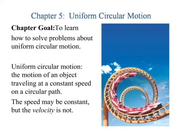
Review: Uniform Circular Motion. In Part 2 we looked at uniform circular motion: r = constant (def. of circular motion) q = t ( q changes with time at uniform rate where w = constant ) v r = 0 (radius doesn’t change) v q = w r (where w = Dq/D t)

E N D
Review:Uniform Circular Motion In Part 2 we looked at uniform circular motion: r = constant (def. of circular motion) q = t (qchanges with time at uniform rate where w = constant) vr = 0 (radius doesn’t change) vq = wr (where w = Dq/Dt) ar = w2r (v changes direction toward center) aq = 0 (angular speed doesn’t change)
Angular Acceleration Here we generalize circular motion to include the case where the angular speed can change. We define angular acceleration as: a = Dw/Dt . [Recall arclength = s, and =s/r, so s=r, vq=r] Since aq = Dvq/Dt = D(wr)/Dt = r(Dw/Dt) = ar. We still have all the equations we had before, except aq is no longer zero but is instead ar.
NON-uniform Circular MotionRectangular viewpoint Circular motion is defined by: r = constant. We still have d/dt = w, but w is no longer held constant. This means that dw/dt = a rather than zero. Converting polar to rectangular, we have: x = r cos(q) = rcos[q(t)] y = r sin(q) = r sin[q(t)] .
Non-uniform Circular MotionRectangular viewpoint x = r cos[q(t)] y = r sin[q(t)] Now we use: vx = dx/dt and vy = dy/dt: vx = dx(t)/dt = dx(q)/dq * dq/dt = r (- sin(q) ) * w = -w r sin(q) vy = dy(t)/dt = dy(q)/dq * dq/dt = r (+ cos(q) ) * w = w r cos(q)
Non-uniform Circular MotionRectangular viewpoint x = r cos(q) y = r sin(q) vx = -w r sin(q) This v is same as for vy = w r cos(q) uniform circular motion Now we use: ax = dvx/dt and ay = dvy/dt. Since w is not constant, we need to use the product rule. ax = - a r sin(q) + -w2r cos(q) ay = +a r cos(q) + -w2r sin(q) .
Non-uniform Circular MotionBack to Polar To convert back to polar for position, we use the inverse transformation equations: x = r cos(q) y = r sin(q) r = [x2 + y2]1/2 = [r2 cos2(q) + r2 sin2(q)]1/2 = r[cos2(q) + sin2(q)]1/2 = r q = inv tan[y/x] = inv tan[ r sin(q) / r cos(q)] = inv tan[tan(q)] = q .
Non-uniform Circular MotionBack to Polar To convert back to polar for velocity, we use the inverse transformation equations: vx = -w r sin(q) vy = w r cos(q) v = [vx2 + vy2]1/2 = [w2r2 sin2(q) + w2r2 cos2(q)]1/2 = wr[sin2(q) + cos2(q)]1/2 = wr qv = inv tan[vy/vx] = inv tan[wr cos(q) / -wr sin(q)] Note that cos(q) = sin(q+90o) and –sin(q) = cos(q+90o) so qv = q 90o.Note that the direction of the velocity, qv, is perpendicular to the direction of the position (the radius), which means the velocity is tangent to the circle.
Non-uniform Circular MotionBack to Polar qv = q 90o Note that the direction of the velocity, qv, is perpendicular to the direction of the position (the radius), which means the velocity is tangent to the circle.
Non-uniform Circular MotionBack to Polar To convert acceleration: ax = - ar sin(q) + -w2r cos(q) ay = +ar cos(q) + -w2r sin(q) . a=[ax2+ay2]1/2 = [a2r2 sin2(q) + 2aw2r2sin(q)cos(q) + w4r2 cos2(q) + a2r2 cos2(q) - 2aw2r2sin(q)cos(q) + w4r2 sin2(q)]1/2 = [(ar)2 + (w2r)2]1/2= [at2+ar2]1/2. We can identify (w2r) as the radial acceleration - due to the turning of the velocity, and we now identify (ar) as the tangential acceleration - due to the changing speed of the velocity.
Non-uniform Circular MotionBack to Polar ax = - ar sin(q) + -w2r cos(q) ay = +ar cos(q) + -w2r sin(q) . a=[at2+ar2]1/2 where at = ar and ar = w2r. If we look at just the ar terms, then the direction of these terms is: qat = inv tan[ cos(q) / -sin(q) ] = q+/- 90o (just like for qv which is tangentto the circle), And if we look just at the w2r terms, then the direction of these terms is: qar = inv tan[ -sin(q) / -cos(q) ] q+/- 180o (which is towards the center).
Constant Angular Acceleration In the special case of constant angular acceleration (a = constant), we have equations analogous to those we had for constant (regular) acceleration: dw/dt = a = constant becomes o dw = t=0ta dt, or w = wo + atlike vx = vxo + axt. dq/dt = w becomes o dq = t=0tw dt = t=0t (wo+at)dt , or q = qo + wot + (1/2)at2like x = xo+vxot+(1/2)axt2.
Constant Angular Acceleration If a car rolls on wheels that do not slip, we can relate the motion of the car to the spinning of the wheels: s = distance of car = arclength of wheels, v = speed of car = v of wheels, a = acceleration of car = a of wheels; q = angle of wheel, w = angular speed of wheel, and a = angular acceleration of wheel:
Constant Angular Acceleration For circular motion: s = rq, r = constant (circular) v = rw = vq vr=0 a = ra = aq ar = w2r (due to turning) For constant acceleration: s = so + vot + (1/2)at2 v = vo + at q = qo + wot + (1/2)at2w = wo + at . This gives many relations so that, by knowing just a few things, we can solve for many other things about the motion.
ExampleConstant Angular Acceleration Consider a car that accelerates from rest to a speed of 20 m/s (45 mph) in 10 seconds on wheels (tires) of outside diameter 66 cm. Assume that the tires roll nicely and do not slip on the road. Through what angle (θ) do the tires rotate during the 10 seconds? What is the final angular speed (ω) at the 10 second mark? What is the angular acceleration (α) of the wheels during the 10 seconds?
Example We can use the equations for constant angular acceleration, or we can use the relations between distance and angle. t = 10 secondsx = ? v = 20 m/s xo= 0 m vo = 0 m/s α = ? θ = ? ω = ? θo = 0 rad ωo = 0 rad/sec d = 66 cm, r = d/2 = 33 cm
Example Since the car is rolling (and not slipping), we recognize that x = s = rθ, and that v = vq= rw . Using the equations for constant angular acceleration along with rw = vq : • = qo + wot + (1/2)at2w = wo + at v = 20 m/s, t = 10 sec., qo = 0rad, r = .33 m, vo = 0 m/s, so wo = 0 rad/sec.
Example • rw = vq becomes: .33 m * w = 20 m/s • q = qo + wot + (1/2)at2 becomes q = 0 + 0 + (1/2)*a*(10 sec)2 (3) w = wo + atbecomes: w = 0 + a*(10 sec) From Eq. 1: w = (20 m/s) / .33 m = 60.6 rad/s From Eq. 3: a = w/t = (60.6 rad/s) / 10 sec = 6.06 rad/s2. From Eq. 2: q = (1/2)*a*(10 sec)2 = (1/2)*(6.06 rad/s2)*(10 sec)2 = 303 rad * (1 cycle/2p rad) = 48.2 revolutions
Example – another way Instead of using the constant angular acceleration formulas, we could solve the regular motion and use the relations between regular quantities and angular quantities: s = rq, r = constant (circular) v = rw = vq vr=0 a = ra = aq ar = w2r (due to turning)
Example another way s = rq, r = constant (circular) v = rw = vq vr=0 a = ra = aq ar = w2r (due to turning) s = so + vot + (1/2)at2 v = vo + at 20 m/s = 0 + a*(10 sec), so a = (20 m/s) / (10 s) = 2 m/s2 , so a = ar, or a = a/r = (2 m/s2) / (.33 m) = 6.06 rad/s2 . s = 0 + 0 + (1/2)*a*(10 sec)2 = (1/2)*(6.06 rad/s2)*(10 sec)2 = 303 radians. v = wr, or w = v/r = (20 m/s) / (.33 m) = 60.6 rad/s.
Rotational Kinematics The computer homework program, Rotational Kinematics, Volume 2 #7, contains explanations and problems involving Rotational Kinematics using the equations in the previous slide.
Rotational Force (Torque) • Forces cause change in the motion, but in Part 2 we only considered motion that changes the position of the object. • What about changing the “spin” or rotation of an object? • To get a nice introduction to the idea of torque, see the computer homework program on Introduction to torque (Vol.2 #5), and continue with the next slide.
Torque There are two important quantities in torque: Force and where you apply the force (called radius). t = r x F = r F sin(qrF) To get a large torque, we need to use a large radius, a large force, and apply the force perpendicular to the radius!
Statics and Torque Just as S F = 0 when the object is static, so also S t = 0 when the object is not spinning (or spinning at a constant rate). In static cases, there is no obvious center to measure the radius from, so we are free to choose any point. However, some points may be simpler to use than others.
Your elbow Let’s consider as an example of torque how your muscles, bones and joints work. Consider holding up a ball of weight 5 lb. How does this work? First we draw a diagram: biceps triceps weight = elbow rw rb
Your elbow In terms of forces and distances, the diagram looks like this: Estimate the distance from your elbow joint FcFb to your biceps connect point, rb, and to your hand, rw. rc=0rbrw W
Your elbow • If the ball weights 5 lb, how much force does your biceps pull up with? How much force of contact does your upper arm push down with on your lower arm at the elbow? • What is the basic principle to use? Statics: S F = 0and S t = 0.
Your elbow From S F = 0 we have: -Fc + Fb - W = 0 And from S t = 0 and measuring from the elbow gives: Fc*rc + Fb*rb - W*rw = 0 . We have two equations and we have two unknowns (Fc and Fb).
Your elbow • We can use the torque equation first, since rc=0 eliminates one of the unknowns, Fc. Fc*rc + Fb*rb - W*rw = 0or Fb = W*rw/rb . • Then we can use the force equation to find Fc : -Fc + Fb - W = 0, or Fc = Fb - W.
Your elbow • By putting in reasonable values for rb and rw, you can see that the biceps have to exert a large force to hold up a relatively light weight! • What advantage does this give? Note how far the biceps have to contract in order to move the weight! This is the advantage of the elbow set-up! • In practice, we use clubs and rackets to make this difference even greater!
Car going around a turn:Sliding off the road or flipping over For a car going around a turn, if the car goes too fast the car will either slide off the road or flip over. What determines which will occur, and how fast can the car go around the turn without either happening? Since we now introduce “flipping over”, we have to consider rotational motion, and hence consider torque. This means we need to consider not only what the forces are, but where they act.
Sliding or Flipping We’ll consider a car making a right turn on an unbanked (horizontal) turn. We have the weight of the car (W=mg), which acts at the center of gravity. We have the contact force, which acts on each of the left and right wheels at the road: FcLand FcR. We have the friction force, which also acts on each of the left and right wheels at the road: FfL and FfR, where Ff mFc We also have an acceleration to the right: ac = v2/r .
Sliding or Flipping The weight, W=mg, acts at the center of gravity, which is at a height, h, above the road. The contact forces, Fc act at the tires which are on the road. The friction forces, Ff, also act at the road. The tires are a distance, w, apart. ac = v2/r h w
Sliding or Flipping SFx = FfL + FfR = m v2/r SFy = FcL + FcR - mg = 0 Let’s choose to consider the center of gravity as the point for rotations. The distances for the torques need to be distances that are to the direction of the forces. We will also choose clockwise as positive for torques. ac = v2/r h w
Sliding or Flipping SFx = FfL + FfR = m v2/r SFy = FcL + FcR - mg = 0 St = -FfL*h - FfR*h + FcL*(w/2) - FcR*(w/2) + mg*0 = 0. Since the FcL is the only force causing a + torque, it must increase and FcR must decrease if the St = 0. This can happen until FcR= 0 and FcL = mg. When this happens, FfR= 0 . ac = v2/r h w
Sliding or Flipping SFx = FfL + 0 = m v2/r, or FfL = mv2/r SFy = FcL + 0 - mg = 0, or FcL = mg St = -FfL*h - 0*h + FcL*(w/2) - 0*(w/2) + mg*0 = 0, or FfL*h = FcL*(w/2). If friction is maximum (limit for sliding) we have: FfL = mv2/r with Ff = mFc = mmg, so mmg = m v2/r, or vmax = [mgr]1/2 . If flipping is to be prevented we have FfL = mv2/r, FcL=mg, or mv2/r * h = mg*(w/2), or vmax = [grw/2h]1/2 .
Sliding or Flipping vmax = [mgr]1/2 applies when sliding is a concern; vmax = [grw/2h]1/2 applies when flipping over is a concern. Which maximum speed is lower - that tells us the true maximum speed to continue around the turn: If m < w/2h, then sliding is the main concern; if m > w/2h, then flipping is the main concern. For big trucks, h is large, and unless the street is very slick, flipping over will be bigger; for sports cars, h is small and sliding is more of a concern.
Statics and Torque The computer homework program, Statics and Torque, Volume 2 #6, contain explanations and problems dealing with this topic.
Torque and Rotations Forces (when not balanced) cause changes in motion. Torques (when not balanced) cause changes in rotational motion. Forces are related to acceleration by Newton’s Second Law: S F = ma. How are t and a related?
Rotational Dynamics Consider: S F = ma and t = r F sin(qrF) . If we multiply both sides of S F = ma by r sin(qrF) we get: S t = m a r sin(qrF) , but a sin(qra) = aq = ar, so S t = mr2a . If the mass is distributed at various radii, then the mr2 becomes S miri2. We define the moment of inertia be be I = S miri2 so that we have S t = Ia .
Moment of Inertia Note that the moment of inertia relates the torque to the angular acceleration just like the mass relates the force to the regular acceleration. Note that the moment of inertia depends on the mass of the objectand also on the shape of the object.
Moment of Inertia Objects that have most of their mass in the center have smaller moments of inertia than objects that have most of their mass on the outside. Using the calculus, we can replace the summation of small mass pieces with an integral: I = S miri2 becomes I = r2 dm. Each small dm has its own radius, or distance from the axis of rotation, so r is really a function of which dm we are using: r(m).
Moment of Inertia I = r2 dm It is awkward to express r(m). We can, however, use density: r = mass/Volumeto convert dm into r dV. Then the integral is really a Volume integral (triple integral). I = r2r dV Using this, we can derive nice formulas for the moment of inertias of certain shapes:Iring = MR2 Isphere = (2/5)MR2; Icylinder = (1/2)MR2 .
Sphere versus Cylinder axis The blue object in the figures is the side view of a cylinder with the same radius and volume (mass) as the orange object (a sphere). Note that most of the mass is in the same place, but the top and bottom of the sphere must be moved away to provide the corners for the cylinder. Hence, the Moment of Inertia of the cylinder is slighly larger than that of the sphere: Isphere = (2/5)MR2 ; Icylinder = (1/2)MR2 . R
Rotational Energy Now that we have the equivalent of Newton’s Second Law for rotations: S t = Ia , let’s see if we can get a rotational energy. Recall that Work = F ds. If we exert a force to spin an object, the ds becomes a small arc length that is perpendicular to the radius. Recall the definition of an angle in radians: q = s/r, so that ds = r dq. But F times r is torque, so we get: Work = t dq .
Rotational Power Work = t dq The definition of power is: P = dWork/dt, and so for rotations we have: P= dW/dt = d[t dq]/dt = t w. This formula for rotational power is similar to that for regular power: P = F v P = t w.
Rotational Kinetic Energy If something is spinning, it can still not be moving so that it’s regular kinetic energy is zero. However, parts of the object are moving, so there is kinetic energy associated with its spinning. We use three relations we have already developed: KE = ½mv2, vq = wr, and I = miri2 KEtotal= ½mivi2 = ½mi(ri)2 = ½2 miri2 = ½Iw2 . This energy is used in the Conservation of Energy just as any other energy term is used.
Angular Momentum Another important tool in solving problems is Conservation of Momentum. Is there a similar tool for rotations? We already have: p = mvand F = dp/dt. If we multiply both sides of Newton’s Second law by the radius we have (with v = wr): t = r F = r dp/dt = d(r p)/dt = dL/dt where we have defined L = r p, where L is called the Angular Momentum.
Conservation of Angular Momentum St = dL/dt Just like F = dp/dt leads to Conservation of momentum if no external forces are present, so St = dL/dt leads to Conservation of Angular momentum if no external torques are present. Note: p = mv, and L = r p= r mv = r m vq = r m wr = mr2w = Iw.
Angular Momentum In class we will observe several demonstrations about Angular Momentum and talk about its uses in controlling rockets and spinning athletes (divers and gymnasts in particular). We will also show how angular momentum relates to riding bicycles, and how this relates to the spinning earth!
Review of Rotational Equations Basically we replace F with t, m with I, v with w, a with aandp with L (where L is the angular momentum): S F = ma S t = Ia Work = = F ds Work = t dq Power = F v Power = t w KE = (1/2)mv2KErotation = (1/2)Iw2 p = mv L = Iw S F = Dp/DtS t = DL/Dt .