ID : T33C-2436

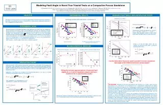
1. Continued Homogeneous deformation 90 90 90 85 N = 1 N = 1 • N = -1 N = 0.71 80 80 N = 0.37 N = 0 80 80 N = 0 N = 0.36 75 N = 0.71 N = -1 70 70 70 70 60 Fault Angle θ Fault Angle θ 65 60 60 Stress N = -1 (AE) 50 60 N = -1 N = 0 (PS) 50 50 55 N = 0 N = 0.37 40 N = 0.37 N = 0.71 Shear band or fault 50 40 40 N = 0.71 N = 1.0 (AC) 30 N = 1.0 45 30 30 0 100 200 300 400 500 Strain 0 100 200 300 400 500 0 100 200 300 400 500 0 100 200 300 400 500 • σ(MPa) σ(MPa) Modeling Fault Angle in Novel True Triaxial Tests on a Compactive Porous Sandstone J. W. Rudnicki1 (847-491-3411; jwrudn@northwestern.edu), Xiaodong Ma2(608-556-4958; xma32@wisc.edu), and Bezalel C. Haimson2(608-262-2563;bhaimson@wisc.edu) 1Dept. Of Civil and Environmental Engineering and Mechanical Engineering, Northwestern University, Evanston, IL 60208 2Dept. of Materials Sci. & Engineering and Geological Engineering Program, University of Wisconsin, Madison, WI 53706 s1at failure s1at failure s1at failure s1at failure s1at failure ID: T33C-2436 Homogeneous deformation Fault Angle θb s2 s1 = s2 Fault Angle θ Stress Stress Stress Stress s2 Stress s2 OBJECTIVE Experimental Results Modeling Fault Angle using Bifurcation Theory s3 = s2 s3 s3 The objective of this research is to evaluate the applicability of the bifurcation theory (Rudnicki & Rice,1975) for predicting the angle of induced fault in high porosity sandstones subjected to three independent principal stresses. Fault angle variation with mean stress  for different N o o o o o Time Variation of μ+ β with  Time Time σ(MPa) Time Time σ(MPa) N = -1 (s2= s1 ） 2.5 (Rough) linear fit 85 • N = 1 (2= 3) From the bifurcation theory: Using a linear fit to the test data of  vs. for N = 0, gives a plausible variation of μ + β with : a roughly linear decrease, except at lower values (below about 200 MPa) where the slope decreases. 2.0 • N = -1 (2= 1) 80 Experimental Work N = 0.37 1.5 • N = 0 (2= (1+3)/2) 75 N = 0.71 1.0 70 b + m Ma and Haimson (see accompanying poster) have conducted true triaxial tests on a compactive porous sandstone (Coconino) using a novel loading path consisting of keeping the minimum compressive stress (3)constant but increasing the other two stresses in a fixed ratio to failure (faulting), thus maintaining constant the deviatoric stress state N. (N is the intermediate principal deviatoric stress divided by . It measures angular position of the stress path in a plane perpendicular to the hydrostat.) For stress ratios 2/1 = 1:1; 1:2; 1:3; 1:6; 0 (where I =i-3,), N varies from -1 (2 =1,axisymmetric extension), to 0 (2=(1 +3)/2, deviatoric pure shear), to 0.36, 0.71 and +1 (2 =3,axisymmetric compression). Both the peak 1 and the angle of fault  were recorded in each test. 0.5 65 Fault Angle θ 60 0.0 N = 0 (Pure Shear) 55 -0.5 N = -1 (AxiSym Ext) N = 0.37 50 -1.0 N = 0.71 45 N = 1 (AxiSym Comp) -1.5 0 100 200 300 400 500 0 100 200 300 400 500 • σ(MPa) σ(MPa) Test data are reasonably represented by a linear regression for each N Experimental data Using μ + β from the Figure above, one can compute the theoretical fault angle busing the following relationships: BI-LINEAR EMPIRICAL MODELING N= 1 (s2= s3 ） N = 0.71 (Ds2/Ds1= 1/6 ） Variation of the intercept,  at  = 0, with N Variation of linear regression slopes with N N = 0 (Ds2/Ds1= 1/2 ） N = 0.37 (Ds2/Ds1= 1/3 ） s3 s3 86 -0.060 -0.065 84 -0.070 82 -0.075 • Slopes of the linear regressions • Expected θ at  = 0 -0.080 80 • Not included -0.085 Can the bifurcation theory be used to predict Coconino sandstone fault angle under different deviatoric stress states? BifurcatioN Theory -0.090 78 -0.095 • Not included 76 Rudnicki and Rice (1975) analyzed deformation localization as a bifurcation from homogeneous deformation. They employed a constitutive relation with a yield function and plastic potential depend that depend on only the first two invariants of stress. The theory leads to prediction of the angle bof shear band or fault upon brittle failure of rock (bis the angle between 1 and the normal to the fault). Application of the theory here is based on an inferred dependence of the sum of a friction coefficient μ and dilatancyfactor β on  for a given N. -0.100 -1.5 -1.0 -0.5 0.0 0.5 1.0 1.5 -1.0 -0.5 0.0 0.5 1.0 N N Fitting the bi-linear approximations of expected fault angles at  = 0, and of regression slopes, both as a function of N, to experimental results: This expression is a rearrangement of the expression for b which can be expressed as: The answer: Predictions of the fault angle based on the variation of μ + βwith  agree well with observations for N= 0.36 and N= 0.71. Predictions for N = 1 (axisymmetric compression) are slightly offset from the line fitted to the data. For N = -1 (axisymmetric extension) the predictions do not agree well with data. For higher mean stress (between 300 and 500 MPa), predicted angles are similar to experimental data, but not so for lower . At  below 200 MPa the theory predicts a dilation band (perpendicular to least compressive stress). Although the observed fault angles increase as the mean stress drops (70 to 80 degrees), the failure is still a shear fault. The reason for these discrepancies is unclear. One possibility is that predictions are based on a two-invariant (oct and ) description of non-elastic behavior. A three-invariant description may improve predictions but introduces additional parameters that are only loosely constrained by the data. Another possibility is that axisymmetric extension and compression are anomalous deformation states in the sense that they do not contain a non-deforming plane that facilitates the formation of a fault. This is the source of known deficiencies of this theory for smooth yield surface models and axisymmetric deformation states (Rudnickiand Rice, 1975). This bi-linear empirical relationship fits data well, except for the axisymmetric compression case (N = 1), which was not used in the linear fitting of experimental data, (see above).