Outline Chapter 6
Schaum’s Outline PROBABILTY and STATISTICS Chapter 6 ESTIMATION THEORY Presented by Professor Carol Dahl Examples from D. Salvitti J. Mazumdar C. Valencia. Outline Chapter 6. Trader in energy stocks random variable Y = value of share want estimates µ y , σ Y

Outline Chapter 6
E N D
Presentation Transcript
Schaum’s OutlinePROBABILTY and STATISTICS Chapter 6 ESTIMATION THEORYPresented by Professor Carol DahlExamples from D. Salvitti J. Mazumdar C. Valencia
Outline Chapter 6 • Trader in energy stocks • random variable Y = value of share • want estimates µy, σY • Y = ß0 + ß1X+ • want estimates Ŷ, b0, b1 • Properties of estimators • unbiased estimates • efficient estimates
Outline Chapter 6 • Types of estimators • Point estimates • µ = 7 • Interval estimates • µ = 7+/-2 • confidence interval
Outline Chapter 6 • Population parameters and confidence intervals Means Large sample sizes Small sample sizes • Proportions • Differences and Sums • Variances • Variances ratios
Properties of Estimators - Unbiased Unbiased Estimator of Population Parameter estimator expected value = to population parameter
Unbiased Estimates Population Parameters: Sample Parameters: are unbiased estimates Expected value of standard deviation not unbiased
Properties of Estimators - Efficient • Efficient Estimator – if distributions of two statistics same more efficient estimator = smaller variance efficient = smallest variance of all unbiased estimators
Unbiased and Efficient Estimates Target Estimates which are efficient and unbiased Not always possible often us biased and inefficient easy to obtain
Types of Estimates for Population Parameter Point Estimate single number Interval Estimate between two numbers.
Estimates of Mean – Known VarianceLarge Sample or Finite with Replacement • X = value of share • sample mean is $32 • volatility is known σ2 = $4.00 • confidence interval for share value • Need • estimator for mean • need statistic with • mean of population • estimator
Estimates of Mean- Sampling Statistic • P(-1.96 < <1.96) = 95% 2.5%
Confidence Interval for Mean • P(-1.96 < <1.96) = 95% • P(-1.96 < <1.96 ) = 95% • P(-1.96 -X < -µ <1.96 - X ) = 95% • Change direction of inequality • P(+1.96 +X > µ > -1.96 + X ) = 95%
Confidence Interval for Mean • P(+1.96 +X > µ > -1.96 + X ) = 95% • Rearrange • P(X - 1.96 < µ <X + 1.96 ) = 95% • Plug in sample values and drop probabilities • X = value of share, sample = 64 • sample mean is $32 • volatility is σ2 = $4 • {32 – 1.96*2/64, 32 + 1.96*2/64} = {31.51,32.49}
Estimates for Mean for Normal • Take a sample • point estimate • compute sample mean • interval estimate – 0.95 (95%+) = (1 - 0.05) • X +/-1.96 • X +/-Zc • (Z<Zc) = 0.975 = (1 – 0.05/2) • 95% of intervals contain • 5% of intervals do not contain
Estimates for Mean for Normal • interval estimate – 0.95 (95%+) = (1 - 0.05) • X +/-Zc • (Z<Zc) = 0.975 = (1 – 0.05/2) • interval estimate – (1-) % • X +/-Zc • (Z<Zc) = (1 – /2) • % of intervals don’t contain • (1- )% of intervals do contain (Z<Zc) = 0.975 = (1 – 0.05/2)
Confidence Interval Estimatesof Population Parameters Common values for corresponding to various confidence levels used in practice are:
Confidence Interval Estimatesof Population Parameters Functions in EXCEL Menu Click on Insert Function or =confidence(,stdev,n) =confidence(0.05,2,64)= 0.49 X+/-confidence(0.05,2,64) =normsinv(1-/2) gives Zc value X+/-normsinv(1-/2) 32 +/- 1.96*2/64
Confidence Intervals for MeansFinite Population (N) no Replacement Confidence interval Confidence level
Example: Finite Population without replacement Evaluate density of oil in new reservoir 81 samples of oil (n) from population of 500 different wells samples density average is 29°API standard deviation is known to be 9 °API = 0.05
Confidence Intervals for MeansFinite Population (N) no ReplacementKnown Variance X = 29 , N= 500, n = 81 , σ = 9 , = 0.05 Zc = 1.96
But don’t know Variance t-Distribution =N(0.1) = = tdf 2/df df
Confidence Intervals of MeansNormal compared to t- distribution t distribution Normal X +/-Zc X +/-tc
Confidence Interval Unknown Variance Example: Eight independent measurements diameter of drill bit 3.236, 3.223, 3.242, 3.244, 3.228, 3.253, 3.253, 3.230 99% confidence interval for diameter of drill bit X +/-tc
Confidence Intervals for MeansUnknown Variance X +/-tc X = ΣXi/n 3.236+3.223+3.242+3.244+3.228+3.253+3.253+3.230 8 X = 3.239 ŝ2 = Σ(Xi - X) = (3.236- X)2 + . . .(3.230 - X)2 (n-1) (8-1) ŝ = 0.0113
Confidence Intervals for MeansUnknown Variance X +/-tc • X = 3.239, n = 8, ŝ= 0.0113, =0.01, • 1- /2=0.995 • From the t-table with 7 degrees of freedom, we find tc= t7,0.995=3.50 1-/2=.975 .005% -tc tc Find tc from Table of Excel
Confidence Intervals for MeansUnknown Variance 1-/2=.975 /2= 0.005% Depends on Table -tc tc GHJ /2 = 0.005 tc = 2. 499 Schaums 1- /2 = 0.995 tc = 2.35 Excel =tinv(0.01,7) = 3.499483
Confidence Intervals for MeansUnknown Variance X +/-tc X = 3.239, n = 8, ŝ= 0.0113, =0.01,
Confidence Intervals for Proportions Example 600 engineers surveyed 250 in favor of drilling a second exploratory well 95% confidence interval for proportion in favor of drilling the second well Approximate by Normal in large samples Solution: n=600, X=250 (successes), = 0.05 zc = 1.96 and
Confidence Intervals for Proportions Example 600 engineers surveyed 250 in favor of drilling a second exploratory well. 95% confidence interval for proportion in favor of drilling the second well Approximate by Normal in large samples Solution: n=600, X=250 (successes), = 0.05 zc = 1.96 and
Confidence Intervals for Proportions sampling from large population or finite onewith replacement
Confidence Intervals Differences and SumsKnown Variances Samples are independent
Confidence Interval for Differences and Sums – Known Variance Example sample of 200 steel milling balls average life of 350 days - standard deviation 25 days new model strengthened with molybdenum sample of 150 steel balls average life of 250 days - standard deviation 50 days samples independent Find 95% confidence interval for difference μ1-μ2
Confidence Intervals for Differences and Sums Example Solution: X1=350, σ1=25, n1=200, X2=250, σ2=50, n2=150
Confidence Intervals for Differences and Sums – Large Samples Where: P1, P2 two sample proportions, n1, n2 sizes of two samples
Confidence Intervals for Differences and Sums Example random samples 200 drilled holes in mine 1, 150 found minerals 300 drilled holes in mine 2, 100 found minerals c Construct 95% confidence interval difference in proportions Solution: P1=150/200=0.75, n1=200, P2=100/300=0.33,n2=300 With 95% of confidence the difference of proportions {0.42, 0.08}
Confidence Intervals Differences and Sums Example Solution: P1=150/200=0.75, n1=200, P2=100/300=0.33, n2=300 95% of confidence the difference of proportions [0.08,0.42]
Confidence Intervals for Variances Need statistic with population parameter 2 estimate for population parameter ŝ2 its distribution - 2
Confidence Intervals for Variances has a chi-squared distribution n-1 degrees of freedom. Find interval such that σ lies in the interval for 95% of samples 95% confidence interval
Confidence Intervals for Variances Rearrange Take square root if want confidence interval for standard deviation
Confidence Intervals for Variances and Standard Deviations Drop probabilities when substitute in sample values 1 - confidence interval for variance 1 - confidence interval for standard deviation
Confidence Intervals for Variance Example Variance of amount of copper reserves 16 estimates chosen at random ŝ2 = 2.4 thousand million tons Find 99% confidence interval variance Solution: ŝ2=2.4, n=16, degrees of freedom = 16-1= 15
How to get 2Critical Values Not symmetric /2 /2 2 lower 2 upper
How to get 2Critical Values 1-/2 Not symmetric 1-/2 /2 /2 GHJ area above 20.995, 20.005 4.60092, 32.8013 Schaums area below 20.005, 20.995 4.60, 32.8 Excel = chiinv(0.995,15) = 4.60091559877155 Excel = chiinv(0.005,15) = 32.8013206461633
Confidence Intervals for Variances and Standard Deviations Example 99% confidence interval variance of reserves Solution: ŝ=2.4 (n-1)=15 2lower = 4.60, 2upper = 32.8
Confidence Intervals for Ratio of Variances Two independent random samples size m and n population variances estimated variances ŝ21, ŝ22 • interested in whether variances are the same • 21/ 22
Confidence Intervals for Ratio of Variances Need statistic with population parameter 21/ 22 estimate for population parameter ŝ21/ ŝ22 its distribution - F
F-Distribution df1 df2
Confidence Intervals for Ratio of Variances Need statistic with population parameter 21/ 22 estimate for population parameter ŝ21/ ŝ22 its distribution - F

