Lexical Analysis (II)
Lexical Analysis (II). Compiler Baojian Hua bjhua@ustc.edu.cn. Recap. lexical analyzer. character sequence. token sequence. Lexer Implementation. Options: Write a lexer by hand from scratch Automatic lexer generator

Lexical Analysis (II)
E N D
Presentation Transcript
Lexical Analysis (II) Compiler Baojian Hua bjhua@ustc.edu.cn
Recap lexical analyzer character sequence token sequence
Lexer Implementation • Options: • Write a lexer by hand from scratch • Automatic lexer generator • We’ve discussed the first approach, now we continue to discuss the second one
Lexer Implementation declarative specification lexical analyzer
Regular Expressions • How to specify a lexer? • Develop another language • Regular expressions, along with others • What’s a lexer-generator? • Finite-state automata • Another compiler…
Lexer Generator History • Lexical analysis was once a performance bottleneck • certainly not true today! • As a result, early research investigated methods for efficient lexical analysis • While the performance concerns are largely irrelevant today, the tools resulting from this research are still in wide use
History: A long-standing goal • In this early period, a considerable amount of study went into the goal of creating an automatic compiler generator (aka compiler-compiler) declarative compiler specification compiler
History: Unix and C • In the mid-1960’s at Bell Labs, Ritchie and others were developing Unix • A key part of this project was the development of C and a compiler for it • Johnson, in 1968, proposed the use of finite state machines for lexical analysis and developed Lex [CACM 11(12), 1968] • Lex realized a part of the compiler-compiler goal by automatically generating fast lexical analyzers
The Lex-like tools • The original Lex generated lexers written in C (C in C) • Today every major language has its own lex tool(s): • flex, sml-lex, Ocaml-lex, JLex, C#lex, … • One example next: • written in flex (GNU’s implementation of Lex) • concepts and techniques apply to other tools
FLex Specification • Lexical specification consists of 3 parts (yet another programming language): Definitions (RE definitions) %% Rules (association of actions with REs) %% User code (plain C code)
Definitions • Code fragments that are available to the rule section • %{…%} • REs: • e.g., ALPHA [a-zA-Z] • Options: • e.g., %s STRING
Rules • Rules: • A rule consists of a pattern and an action: • Pattern is a regular expression. • Action is a fragment of ordinary C code. • Longest match & rule priority used for disambiguation • Rules may be prefixed with the list of lexers that are allowed to use this rule. <lexerList> regularExp {action}
Example %{ #include <stdio.h> %} ALPHA [a-zA-Z] %% <INITIAL>{ALPHA} {printf (“%c\n”), yytext);} <INITIAL>.|\n => {} %% int main () { yylex (); }
Lex Implementation • Lex accepts REs (along with others) and produce FAs • So Lex is a compiler from REs to FAs • Internal: table-driven algorithm RE NFA DFA
M Input String {Yes, No} Finite-state Automata (FA) M = (, S, q0, F, ) Transition function Input alphabet State set Final states Initial state
Transition functions • DFA • : S S • NFA • : S (S)
a a 0 1 2 b b a,b DFA example • Which strings of as and bs are accepted? • Transition function: • { (q0,a)q1, (q0,b)q0, (q1,a)q2, (q1,b)q1, (q2,a)q2, (q2,b)q2 }
a,b 0 1 b a b NFA example • Transition function: • {(q0,a){q0,q1}, (q0,b){q1}, (q1,a), (q1,b){q0,q1}}
RE -> NFA:Thompson algorithm • Break RE down to atoms • construct small NFAs directly for atoms • inductively construct larger NFAs from smaller NFAs • Easy to implement • a small recursion algorithm
RE -> NFA:Thompson algorithm e -> -> c -> e1 e2 -> e1 | e2 -> e1* c e2 e1
RE -> NFA:Thompson algorithm e -> -> c -> e1 e2 -> e1 | e2 -> e1* e1 e2 e1
Example alpha = [a-z]; id = {alpha}+; %% ”if” => (…); {id} => (…); /* Equivalent to: * “if” | {id} */
Example ”if” => (…); {id} => (…); f i …
NFA -> DFA:Subset construction algorithm (* subset construction: workList algorithm *) q0 <- e-closure (n0) Q <- {q0} workList <- q0 while (workList != []) remove q from workList foreach (character c) t <- e-closure (move (q, c)) D[q, c] <- t if (t\not\in Q) add t to Q and workList
NFA -> DFA:-closure /* -closure: fixpoint algorithm */ /* Dragon book Fig 3.33 gives a DFS-like * algorithm. * Here we give a recursive version. (Simpler) */ X <- \phi fun eps (t) = X <- X ∪ {t} foreach (s \in one-eps(t)) if (s \not\in X) then eps (s)
NFA -> DFA:-closure /* -closure: fixpoint algorithm */ /* Dragon book Fig 3.33 gives a DFS-like * algorithm. * Here we give a recursive version. (Simpler) */ fun e-closure (T) = X <- T foreach (t \in T) X <- X ∪ eps(t)
NFA -> DFA:-closure /* -closure: fixpoint algorithm */ /* And a BFS-like algorithm. */ X <- empty; fun e-closure (T) = Q <- T X <- T while (Q not empty) q <- deQueue (Q) foreach (s \in one-eps(q)) if (s \not\in X) enQueue (Q, s) X <- X ∪ s
4 8 Example ”if” => (…); {id} => (…); f i 1 2 3 0 [a-z] 5 6 7 [a-z]
4 8 Example q0 = {0, 1, 5} Q = {q0} D[q0, ‘i’] = {2, 3, 6, 7, 8} Q ∪= q1 D[q0, _] = {6, 7, 8} Q ∪= q2 D[q1, ‘f’] = {4, 7, 8} Q ∪= q3 f i 1 2 3 0 [a-z] 5 6 7 f q1 q3 i _ [a-z] q0 q2
4 8 Example D[q1, _] = {7, 8} Q ∪= q4 D[q2, _] = {7, 8} Q D[q3, _] = {7, 8} Q D[q4, _] = {7, 8} Q f i 1 2 3 0 [a-z] 5 6 7 f q3 q1 _ [a-z] i _ _ _ q0 q4 _ q2
4 8 Example q0 = {0, 1, 5} q1 = {2, 3, 6, 7, 8} q2 = {6, 7, 8} q3 = {4, 7, 8} q4 = {7, 8} f i 1 2 3 0 [a-z] 5 6 7 f q3 letter [a-z] q1 i letter-f q4 q0 letter letter q2 letter-i
4 8 Example q0 = {0, 1, 5} q1 = {2, 3, 6, 7, 8} q2 = {6, 7, 8} q3 = {4, 7, 8} q4 = {7, 8} f i 1 2 3 0 [_a-zA-Z] 5 6 7 f q3 letter q1 [_a-zA-Z0-9] i letter-f q4 q0 letter letter q2 letter-i
DFA -> Table-driven Algorithm • Conceptually, an FA is a directed graph • Pragmatically, many different strategies to encode an FA in the generated lexer • Matrix (adjacency matrix) • sml-lex • Array of list (adjacency list) • Hash table • Jump table (switch statements) • flex • Balance between time and space
Example: Adjacency matrix ”if” => (…); {id} => (…); f q3 letter q1 i letter-f q4 q0 letter letter q2 letter-i
DFA Minimization:Hopcroft’s Algorithm (Generalized) f q3 letter q1 i letter-f q4 q0 letter letter q2 letter-i
DFA Minimization:Hopcroft’s Algorithm (Generalized) f q3 letter q1 i letter-f q4 q0 letter letter q2 letter-i
DFA Minimization:Hopcroft’s Algorithm (Generalized) f q3 q1 i letter letter-f q0 q2, q4 letter-i letter
Summary • A Lexer: • input: stream of characters • output: stream of tokens • Writing lexers by hand is boring, so we use lexer generators • RE -> NFA -> DFA -> table-driven algorithm • Moral: don’t underestimate your theory classes! • great application of cool theory developed in mathematics. • we’ll see more cool apps. as the course progresses