Download

1 / 35
350 likes | 444 Views
Explore the dynamic property of entanglement in quantum states regarding time and space, with insights into noise impact, spatial localization, and quantum memory forces. Discover the behavior of entangled atoms in decay and molecular dissociation scenarios.

E N D
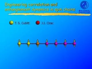
Quantum Optics II Cozumel, Mexico, December 5-8, 2004 • ”Entanglement in Time and Space” • J.H. Eberly, Ting Yu, K.W. Chan, and M.V. Fedorov • University of Rochester / Prokhorov Institute • We consider entanglement as a dynamic property of quantum states and examine its behavior in time and space. Some interesting findings: (1) adding more noise helps fight phase-noise disentanglement, and (2) high entanglement induces spatial localization, equivalent to a quantum memory force. • Ting Yu & JHE, Phys. Rev. Lett. 93, 140404 (2004). • K.W. Chan, C.K. Law and JHE, Phys. Rev. Lett. 88, 100402 (2002) • JHE, K.W. Chan and C.K. Law, Phil. Trans. Roy. Soc. London A 361, 1519 (2003). • M.V. Fedorov, et al., Phys. Rev. A 69, 052117 (2004).
Superposition of conflicting information, but only one object. Can you handle the conflictinginformation here? Which face is in the back? Entanglement means a superposition of conflicting information about two objects.
A pair of conflicts can be “entangled” Try to see both at the same time. Do they “flip” together?
Measurement cancels contradiction A pair of boxes, but only one view of them
Bell States provide a simple example Schrödinger-cat “Bell State”: |-> =|C*>|N*> + |C>|N> excited cat = C*, dead cat = C, excited nucleus = N*, ground state = N
Bell States provide a simple example Schrödinger-cat “Bell State”: |-> =|C*>|N*> + |C>|N> excited cat = C*, dead cat = C, excited nucleus = N*, ground state = N <N|-> = |C> (sorry, Cat)
Overview Issue-- entanglement in time and space. Illustration #1 -- two atoms are excited and entangled but not communicating with each other. Result #1-- both atoms decay, diag e-2gt and off-diag e-gt , just as expected; but entanglement of the atoms behaves qualitatively differently. Illustration #2 -- two atoms fly apart in molecular dissociation. Result #2-- entanglement means localization in space (a “quantum memory force”). For detailed treatments: Ting Yu & JHE, PRL 93 140404 (2004), and M.V. Fedorov, et al., PRA 69, 052117 (2004).
A B HAT = (1/2)wAsZA + (1/2)wBsZB , HCAV = kwkak†ak + knkbk†bk HINT = k(gk*s-Aak† + gks+Aak) + k(fk*s-Bbk† + fks+Bbk) At t=0 the joint initial state rABis entangled and mixed (not pure). The atoms only decay (no cavity feedback). After t=0, what happens to entanglement? Illustration #1:
++ +- -+ -- ++ a 0 0 0 +- 0 1 1 0 -+ 0 1 1 0 -- 0 0 0 d Initial state, entangled and mixed, where d = 1-a. r = C = concurrence EOF concurrence 1 ≥ C ≥ 0 mixedinitial states, C = 2/3
a(t) 0 0 0 0 b(t) z(t) 0 0 z*(t) c(t) 0 0 0 0 d(t) r = a 0 0 0 0 1 1 0 0 1 1 0 0 0 0 d Time Evolution Result: Obvious point: the atoms go to their ground states, so d 3, and the other elements decay to zero. No surprise: the decay of r(t) is smooth, and exponential, measured by usual natural lifetime: s±A(t) = s±A(0) exp[-GAt/2 ± iwAt] Reminder: the atoms decay independently.
(t) = Km(t) r(0) Km†(t) Sol’n. in Kraus representation: Kraus operators: gA = exp[-Gt / 2 ] wA2 = 1- exp[-Gt ] , same for B. for details, see Ting Yu and JHE, PRB 68, 165322 (2003)
r Decays all depend on gA(t) = exp(-GAt/2) and gB(t) = exp(-GBt/2). a(t) = gAgB, b(t) = gB2 +gA2 B2, c(t) = gA2 +gB2 A2, d(t) = A2 +A2 +A2A2, z(t) = gAgB , where A2 = 1 - gA2, etc. a 0 0 0 0 b z 0 0 z* c 0 0 0 0 d Usual Born-Markov solutions for the separate atoms: s±A(t) = s±A(0) exp[-GAt/2 ± iwAt] Kraus matrix evolution: For detailed treatment: Ting Yu & JHE, PRL 93, 140404 (2004).
Entanglement evolution: Entanglement has its own rules, and follows the atom decay law only exceptionally. Entanglement can be completely lost in a finite time! art by Curtis Broadbent Ting Yu & JHE, Phys. Rev. Lett. 93, 140404 (2004).
Noise + Entanglement Werner state density matrix Werner qubits undergo only off-diagonal relaxation under the influence of phase noise. All entanglement of a Werner state is destroyed in a finite time by pure phase noise.
Two Noises + Entanglement Pure off-diagonal relaxation of qubits Add some diagonal relaxation, for example via vacuum fluctuations. Add diag. to off-diag. relaxation of qubits Werner entanglement gets some protection from added noise! Ting Yu & JHE (in preparation).
Experiments following the original EPR “breakup” scenario have not been done yet. Spatial localization and entanglement With just two objects, high entanglement can be reached by allowing each object a wide variety of different states. The idealized two-particle wave function used by Einstein, Podolsky and Rosen in their famous 1935 EPR paper used continuous variables (infinite number of states) to get the maximum degree of entanglement.
Spontaneous emission(K ≈ 1) Chan, Law and Eberly, PRL 88, 100402 (2002) Fedorov, et al. (in preparation, 2004) Raman scattering(K > 100) Chan, Law, and Eberly, PRA 68, 022110 (2003)Chan, et al., JMO 51, 1779 (2004). Ionization/Dissociation(K > 10) Fedorov, et al., PRA 69, 052117 (2004). Chan and Eberly, quant-ph 0404093 Down conversion (K ≈ 4.5 — 1000’s)Huang and Eberly, JMO 40, 915 (1993) Law, Walmsley and Eberly, PRL 84, 5304 (2000)Law and Eberly, PRL 92, 127903 (2004) Physical examples of breakup 17
EPR system is created by break-up The variables entangled are positions (x1and x2), or momenta (k1 and k2). Perfect correlation is implied in the EPR wavefunction: How much correlation is realistic? How to measure it? Original paper: Einstein, Podolsky and Rosen, Phys. Rev. 47, 777 (1935).
All information is in Y. We can plot the two-particle density |Y|2 vs. x1 and x2. • Knowledge of one particle gives information about the other particle. • Joint localization information is packet entanglement. |Y|2 Fedorov ratios for particle localization: We can calculate these for a simple dissociation model. Localization - Entanglement
relative part CM part Time-dependent EPR example Given a dissociation rategd, a post-breakup diatomicYis: M.V. Fedorov, et al., PRA 69, 052117 (2004) / quant-ph/0312119.
Dynamics of localization What do we know and when do we know it? • Massive particles spreading wavepackets: Dx Dx(t) and DX DX(t) • EPR pairs: [x, P] = 0 and [X, p] = 0 nonlocality • Spreading is governed by the free-particle Hamiltonian. • Time evolution is merely via phase in the momentum picture:
Calculation Inferred dependence Dynamics of localization - F ratios Plots of |Y(t)|2 vs. x1 and x2 : Experiments track localization via packet spreading (i.e.,spatial variances). The two-particle ratio h(t) = ∆x/2∆X is a convenient parameter [*]connected with dynamical evolution. * Chan, Law and Eberly, PRL 88, 100402 (2002).
Universal man-in-street theory Model thebreakup state as double-Gaussian [*]. * K.W. Chan and JHE, quant-ph 0404093 This makes it easy to calculate the Fedorov ratios (F1 ~ F2 ) at t=0 and for later times. Question: can we guess what happens to localization?
When these exponents are added, the nonseparablex1x2term 0 at a specific time t0: Entanglement migration to phase Therefore P(x, X; t) = (x, X; t)2has two similar real exponents.
Quantum memory force (QMF) Atom Photon The dissociation example has a close analog in spontaneous emission. These atom-photon space functions show a “force” arising from shared quantum information, a “quantum memory force” (QMF).The first four bound states are shown for Schmidt number K = 3.5, which is slightly “beyond-Bell.,” i.e., K > 2. M.V.Fedorov, et al. (in preparation). Chan-Law-Eberly, PRL 88, 100402 (2002)
Summary / dynamics of entanglement • Entanglement dynamics are largely unknown (time or space) • Noisy environment kills entanglement but not intuitively • Individual atom decay is not a guide for entanglement • Diag. + off-diag. noise has a cancelling effect • EPR-type breakup is ubiquitous / creates two-party correlation • Conditional localization vs. entanglement ? • Packet dynamics, Fedorov ratio and control parameter h • Man-in-street theory and phase entanglement • Memory effects enforce spatial configurations (QMF)
Acknowledgement Research supported by NSF grant PHY-00-72359, MURI Grant DAAD19-99-1-0215, NEC Res. Inst. grant, and a Messersmith Fellowship to K.W. Chan. References Ting Yu & J.H. Eberly, PRL 93, 140404 (2004) and in preparation. M.V. Fedorov, et al., PRA 69, 052117 (2004). C.K. Law and J.H. Eberly, PRL 92, 127903 (2004). M.V. Fedorov, et al., PRA (in preparation). K.W. Chan, C.K. Law and J.H. Eberly, PRL 88, 100402 (2002). K.W. Chan and J.H. Eberly, quant-ph/0404093. A. Einstein, B. Podolsky and N. Rosen, Phys. Rev. 47, 777 (1935).
Size of ent. More sophisticated Schmidt analysis Any bipartite pure state can be written as a single discrete sum: • Continuous basis discrete basis • Unique association of system 1 to system 2 e.g.,
Discretization of continuum information, the Schmidt advantage Unique mode pairs Continuous-mode basis Schmidt-mode basis Pure-state non-entropic measure of entanglement: Schmidt number counts experimental modes, provides practical metric
Interpreting K, the Schmidt number K = 1, no entanglement. K = 2, perfect Bell states. K = 5, beyond Bell, more information. K = 10, still more info. Quantum info is always discrete and countable.
Estimation of K for photodissociation Comparing the photodissociation process with the double-Gaussian model, we identify Dx0 = v ⁄ gd andDX0 = DR0. If we take DR0 = 10 nm, , and define td = gd-1, then with td in sec,
Retreat of entanglement into phase The Fedorov ratios for double-Gaussian : Position: Momentum: where , so . Note non-equivalence of k-space and x-space for these experimentally measurable quantities.
Double-Gaussian Schmidt analysis For the man-in-street double-Gaussian model (with m1 = m2) The Schmidt modes are the number states and one finds: while from the actual wave function we had inferred with h(t) = ∆x(t)/2∆X(t). These are the same, except for spreading!