Download
1 / 32
320 likes | 464 Views
Chapter III Rasterization. Rasterization Stage.

E N D
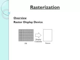
Rasterization Stage • The vertices processed by the vertex program enter a hard-wired stage and are assembled to build primitives such as triangles. Each primitive is further processed to determine its 2D form appearing on the screen, and is rasterized into a set of fragments. • The hard-wired stage is generally named primitive assembly and rasterization. Direct3D simply calls this stage rasterization or rasterizer. • The hard-wired rasterization stage performs the following: • Clipping • Perspective division • Back-face culling • Viewport transform • Scan conversion (rasterization in a narrow sense)
Clipping • Clipping is performed in the clip space, but the following figure presents its concept in the camera space, for the sake of intuitive understanding. • ‘Completely outside’ triangles are discarded. • ‘Completely inside’ triangles are accepted. • ‘Intersecting’ triangles are clipped. • As a result of clipping, vertices may be added to and deleted from the triangle. • Clipping in the (homogeneous) clip space is a little complex but well-developed algorithm.
Perspective Division • Unlike affine transforms, the last row of Mproj is not (0 0 0 1) but (0 0 -1 0). When Mproj is applied to (x,y,z,1), the w-coordinate of the transformed vertex is –z. • In order to convert from the homogeneous (clip) space to the Cartesian space, each vertex should be divided by its w-coordinate (which equals –z).
Perspective Division (cont’d) • Note that –z is a positive value representing the distance from the xy-plane of the camera space. Division by –z makes distant objects smaller. It is perspective division. The result is defined in NDC (normalized device coordinates).
Back-face Culling • The polygons facing away from the viewpoint of the camera are discarded. Such polygons are called back-faces. (The polygons facing the camera are called front-faces.) • In the camera space, the normal of a triangle can be used to determine whether the triangle is a front-face or a back-face. A triangle is taken as a back-face if the camera (EYE) is in the opposite side of the triangle's normal. Otherwise, it is a front-face. • For the purpose, compute the dot product of the triangle normal n and the vector c connecting the camera position and a vertex of the triangle.
Back-face Culling (cont’d) • Unfortunately, back-face culling in the camera space is expensive. • The projection transform makes all the connecting vectors parallel to the z-axis. The universal connecting vector represents the parallelized projection lines. Then, by viewing the triangles along the universal connecting vector, we can distinguish the back-faces from the front-faces.
Back-face Culling (cont’d) • Viewing a triangle along the universal connecting vector is equivalent to orthographically projecting the triangle onto the xy-plane. • A 2D triangle with CW-ordered vertices is a back-face, and a 2D triangle with CCW-ordered vertices is a front-face. • Compute the following determinant, where the first row represents the 2D vector connecting v1 and v2, and the second row represents the 2D vector connecting v1 and v3. If it is positive, CCW. If negative, CW. If 0, edge-on face. • Note that, if the vertices are ordered CW in the clip space, the reverse holds, i.e., the front-face has CW-ordered vertices in 2D.
Back-face Culling – OpenGL Example • OpenGL and Direct3D allow us to control the face culling mechanism based on vertex ordering.
Coordinate Systems – RHS vs. LHS • RHS vs. LHS • Notice the difference between 3ds Max and OpenGL: The vertical axis is the z-axis in 3ds Max, but is the y-axis in OpenGL.
Coordinate Systems – 3ds Max to OpenGL If the scene is exported as is to OpenGL, the objects appear flipped. At the time of export, flip the yz-axes while making the objects immovable.
Coordinate Systems – 3ds Max to Direct3D • Assume that the yz-axes have been flipped. Then, ‘3ds Max to Direct3D’ problem is reduced to ‘OpenGL to Direct3D.’ • Placing an RHS-based model into an LHS (or vice versa) has the effect of making the model reflected by the xy-plane mirror, as shown in (a). • The problem can be easily resolved if we enforce one more reflection, as shown in (b). Reflecting the reflected returns to the original! • Reflection with respect to the xy-plane is equivalent to negating the z-coordinates.
Coordinate Systems – 3ds Max to Direct3D (cont’d) • Conceptual flow from 3ds Max to Direct3D
Coordinate Systems – 3ds Max to Direct3D (cont’d) • Conceptual flow from 3ds Max to Direct3D
Coordinate Systems – 3ds Max to Direct3D (cont’d) • Conversion from 3ds Max to Direct3D requires yz-axis flip followed by z-negation. The combination is simply yz-swap.
Coordinate Systems – 3ds Max to Direct3D (cont’d) • When only yz-swap is done, we have the following image. Instead of back-faces, front-faces are culled. • The yz-swap does not change the CCW order of vertices, and therefore the front-faces have CCW-ordered vertices in 2D. In Direct3D, the vertices of a back-face are assumed to appear CCW-ordered in 2D, and the default is to cull the faces with the CCW-ordered vertices. • The solution is to change the Direct3D culling mode such that the faces with CW-ordered vertices are culled.
Viewport • A window at the computer screen is associated with its own screen space. It is a 3D space and right-handed. • A viewport is defined in the screen space. typedef struct _D3DVIEWPORT9 { DWORD X; DWORD Y; DWORD Width; DWORD Height; float MinZ; float MaxZ; } D3DVIEWPORT9; typedef struct D3D10_VIEWPORT { INT TopLeftX; INT TopLeftY; UINT Width; UINT Height; FLOAT MinDepth; FLOAT MaxDepth; } D3D10_VIEWPORT;
Viewport Transform In most applications, MinZ and MaxZ are set to 0.0 and 1.0, respectively, and both of MinX and MinY are zero.
Scan Conversion • The last substage in the rasterizer is scan conversion, which is often called “rasterization in a narrow sense.” • It defines the screen-space pixel locations covered by the primitive and interpolates the per-vertex attributes to determine the per-fragment attributes at each pixel location.
Top-left Rule • When a pixel is on the edge shared by two triangles, we have to decide which triangle it belongs to. • A triangle may have right, left, top or bottom edges. • A pixel belongs to a triangle if it lies on the top or left edge of the triangle.
Object Picking • An object is picked by placing the mouse cursor on it or clicking it. • Mouse clicking simply returns the 2D pixel coordinates (xs,ys). Given (xs,ys), we can consider a ray described by the start point (xs,ys,0) and the direction vector (0,0,1). • The ray will be transformed back to the world or object space, and then ray-object intersection test will be done. For now, let’s transform the ray to the camera space
Object Picking (cont’d) direction vector of the camera-space ray (CS_Direc)
Object Picking (cont’d) • Let us transform the direction vector of the camera-space ray (CS_Direc) into the world space (WS_Direc). • For now, assume that the start point of the camera-space ray is the origin. Then, the start point of the world-space ray (WS_Start) is simply EYE.
Object Picking (cont’d) • In principle, we have to perform the ray intersection test with every triangle in the triangle list. A faster but less accurate method is to approximate each mesh with a bounding sphere that completely contains the mesh, and then do the ray-sphere intersection test.
Object Picking (cont’d) • Bounding volumes • Bounding volume creation
Object Picking (cont’d) • For the ray-sphere intersection test, let us represent the ray in a parametric representation. • Collect only positive ts. (Given two positive ts for a sphere, choose the smaller.)
Object Picking (cont’d) • The bounding sphere hit first by the ray is the one with the smallest t with the range constrain [n,f].
Object Picking (cont’d) • Ray-sphere intersection test is often performed at the preprocessing step, and discards the polygon mesh that is guaranteed not to intersect the ray.