Download
1 / 68
680 likes | 936 Views
Repetition Multiple imputation. Ziad Taib Biostatistics, AZ May 20, 2009. Data set with missing values. Completed set. Result. General principles. Informal justification. The algorithm (Estimation). Pooling information. MI in practice. A simulation-based approach to missing data.

E N D
RepetitionMultiple imputation Ziad Taib Biostatistics, AZ May 20, 2009 Name, department
Data set with missing values Completed set Result
MI in practice A simulation-based approach to missing data 1. GenerateM > 1 plausible versions of. Complete Cases 2. Analyze each of theMdatasets by standard complete-datamethods. ^ ^ ^ ^ ^ 3. Combine the results across theMdatasets (M =3-5 is usually OK). ^ = imputation for Mth dataset
Software 2. SAS software (experimental) It is part of SAS/STAT version 8.02 SAS institute paper on multiple imputation, gives an example and SAS code: http://www.sas.com/rnd/app/papers/multipleimputation.pdf SAS documentation on PROC MI http://www.sas.com/rnd/app/papers/miv802.pdf SAS documentation on PROC MIANALYZE http://www.sas.com/rnd/app/papers/mianalyzev802.pdf
Software 1. Joe Schafer’s software from his web site. ($0) http://www.stat.psu.edu/%7Ejls/misoftwa.html#top Schafer has written publicly available software primarily for S-plus. There is a stand-alone Windows package for data that is multivariate normal. This web site contains much useful information regarding multiple imputation.
Software 3. SOLAS version 3.0 ($1K) http://www.statsol.ie/solas/solas.htm Windows based software that performs different types of imputation: • Hot-deck imputation • Predictive OLS/discriminant regression • Nonparametric based on propensity scores • Last value carried forward Will also combine parameter results across theManalyses.
MI in SAS has 3 steps Create multiple imputed data sets Analysis task Combine results after analysis MI in SAS
RepetitionPower and sample size estimation Ziad Taib Biostatistics, AZ May 20, 2009 Name, department 14 Date
Example: Estimating the sample size needed in a trial for chronic pulmonary diseases Name, department 15 Chronic pulmonary diseases (such as Chronic Obstructive Pulmonary Disease – COPD) concern the development of emphysema. A clinical trial using lung densitometry (measuring the lung density through CT scan) as an endpoint is typically designed as a longitudinal study with repeated measurements at fixed time intervals. Since lung density measurements are closely correlated with lung volume (inspiration level), it is important to include lung volume measurements in statistical analyses as a longitudinal covariate. Lung volume is normally measured at the same time as the lung density is measured. Date
(1) Name, department 16 The clinical efficacy can be assessed by comparing the progression of lung density loss between two treatment groups (active vs. placebo) using a random coefficient model – a longitudinal linear mixed model with a random intercept and slope. In planning the clinical trial with such complex statistical analyses, the calculation of the sample size required to achieve a given power to detect a specified treatment difference is an important, often complex issue. In this example, an empirical approach is used to calculate the sample size by simulating trajectories of lung density and lung volume using SAS. We present step-by-step details for sample size calculation through simulation, and discuss the pros and cons of this approach. Date
17 Yijis the efficacy endpoint (i.e. lung density) measurement for subject i = 1, 2,…, n, at fixed time point j = 1, 2, …, K. TRT is an indicator of subject i’s treatment group (i.e. TRT=1 for active drug; TRT=0 for placebo). COVij is a longitudinal covariate (i.e. logarithm of lung volume) for subject i = 1, 2,…, n, at fixed time point j = 1, 2, …, K. b0 and b2 are subject-specific random effects for the intercept and slope, respectively, which are from a normal distribution with mean 0 and variance σ02 and σ02, respectively. εij is the random error from a normal distribution with mean 0 and variance σ2. β0, β1, β2, β3, and β4 are the fixed effects for intercept, treatment, time, covariate and interaction of treatment and time respectively. Here we assume that the benefits can be assessed quantitatively by comparing the slopes of lung density trajectories for the two treatment groups. This quantity is captured by β4.
Sample Size Estimation Using Simulations 18 In the model, β4is typically our interest, which is the difference in slope of time between two treatment groups (active vs. placebo). There is no direct mathematical formula to calculate the sample size for a given statistical power (i.e. 80%) to test the null hypothesis: β4=0 with a specified type I error (i.e. α=0.05). One approach to calculate the sample size for a given power is through the simulation. Date
Methods used 19 Assume we know the parameters β0, β1, β2, β3, and β4, and σ02 and σ02 from either history data, previous clinical trialsor meaningful clinical differences. We want to test, the study design in terms of number of time points (K) and fixed time intervals (TIME), and the longitudinal covariate COVij. For a fixed equal sample size n for each treatment, the trajectories of efficacy measurement Yij (i.e. lung density) for the n subjects can be simulated through the model for each treatment group. Then,perform a statistical test on β4 =0by using the SAS Proc MIXED on the simulated data set, and record whether thep-value < 0.05. Date
(*) In reality β4=0.7>0(in our simulations)so the proportion of times we reject the hypothesis β4 =0 of the power. 5. The sample code to perform the test is as follow: proc mixed data = data; class id trt; model y = trt time trt*time cov / solution; random intercept time/ subject = id type = un; run; • For the fixed sample size n per treatment group, simulate M(i.e. M=1000) times and the proportion of significance tests of β4 =0 among the total M simulations is the statistical power (*) for the sample size n per treatment group. • Then, adjust the sample size n to achieve desirable statistical power.
Simulating the response (2) Name, department 21 In order to simulate the trajectories of Yij, it is necessary to simulate the trajectories of longitudinal covariate COVij. Similarly, assume COVij is from a linear model regressing against time with a random intercept Where g0 and g1 are the fixed intercept and slope respectively; r0 and εij are from a normal distribution with mean 0 and variance d12 and d22, respectively. If we know the parameters (g0, g1 , d12 and d22 ) from history data or previous clinical trials for the study population, it will be simple to simulate the trajectories of the longitudinal covariate COVij by using SAS random generating functions Date
22 Date Summary: 1. Obtain the pre-specified parameters through either history data, previous clinical trials or meaningful clinical difference to be tested from clinicians 2. Specify a desired statistical power (i.e. 80%) and a type-1 error rate (i.e. 5%) 3. Simulate trajectories of efficacy measurement (i.e. lung density) and longitudinal covariate (i.e. logarithm of lung volume) for a fixed sample size (n) of subjects within each treatment arm • A. Trajectories of longitudinal covariate (i.e. logarithm of lung volume) are simulated through model (2) • B. Trajectories of efficacy measurement (i.e. lung density) are simulated through model (1)
Name, department 23 4. Perform the statistical test on β4=0 based on the simulated data set. Record whether a p-value < 0.05 was obtained 5. Repeat steps 3 and 4 M (i.e. M=1000) times and calculate the statistical power for the fixed sample size 6. Repeat steps 3 - 5 for various values of n. Stop when desired statistical power is obtained Date
Results: Example of a Simulation Name, department 24 Assume there are two treatment groups (active vs. placebo) in a study design. The efficacy endpoint along with the longitudinal covariate will be measured at K=4 time points at baseline, 1 year, 2 years and 3 years. All corresponding parameters specified in model (1) and (2) could be obtained either through history data, previous clinical trials or meaningful clinical difference to be tested from clinicians. For purpose of simulation, they are randomly selected and specified as below: Date
n Name, department 25 The summary of statistical power for a given sample size per treatment based on M = 1000 simulated data sets is listed below: Therefore, a sample size 45 per treatment arm has an estimated statistical 80% power to detect the treatment slope difference of 0.7 in a random coefficient model for the study design above. Date
Conclusions and Discussion 26 In practice, it is rarely the case that all subjects have the complete data for all visits in the study because of missing certain study visits, drop out or other reasons. Since our simulation framework assumes there are no missing observations, we recommend that the implemented sample size for the designed trial include more subjects than the number estimated from the simulation. In most cases an increase of 5% or 10% should suffice, but depending on the characteristics of the designed trial such as the study population, difficulty of study procedure, difficulty of study measurement etc to cause the subject’s drop out or missing of study measurements. The appropriate percentage could vary. Date
Post-Hoc Power (also known as observed power or retrospective power) • You have collected the data, ran an appropriate statistical analysis, and did not observe statistical significance as indicated by a relatively “large” p-value. So you decide to compute post-hoc power to see how powerful the test was, which, by itself is essentially an empty, meaningless result. • Post-hoc power is merely a one-to-one transformation of the p-value (based on the F-statistic and degrees of freedom as illustrated above). • In this situation power was computed based only on what this particular sample data showed: the observed difference in means, the computed standard error, and the actual sample sizes of the groups all contributed to the observed “power” exactly as they did to the p-value.
… So, power calculations can only be considered as a prospective or an "a priori" concept. Power calculations should be directed towards planning a study, not an after-theexperiment review of the results. • None of the SAS statistical procedures (e.g., PROCs REG, TTEST, GLM, or MIXED and others) provide retrospective (post hoc) power calculations. (However, through saving results from PROC MIXED with the ODS and following through with a few basic SAS functions, it is quite simple to compute them in a DATA step or with the inputs to PROC POWER or PROC GLMPOWER.)
Any Questions? Name, department
Sample Questions for the Final Exam Ziad Taib Biostatistics, AZ MV, CTH Name, department 30 Date
Question 1 31 • Formulate the general LMM and • State its underlying assumptions. • Explain/interpret its ingredients • Explain what is meant by the marginal model • Explain what is meant by the hierarchical model. • Explain the difference between the marginal- and the hierarchical model Date
Question 2 32 Explain how and why the predicted values of the random effects in a linear mixed model can be used to identify outliers Date
Question 3 33 Formulate the generalized linear mixed model and give an example of your choice of its use. Date
Question 4 34 Skiss for how we can obtain a useful formula for the prediction of the random effects. Only a principle description is needed. Date
Question 5 35 Define missing at random and missing completely at random. Argue why the the direct maximum likelihood method can be used under a suitable ignorability condition. Date
Question 6 36 Explain what is meant by Multiple Imputation (MI). Describe the main algorithm used in MI and give a informal argument for why it is valid. Date
Question 7 37 Give two different candidates for the definition of residual in a general LMM. Date
Answers to samplequestion 1 Ziad Taib Biostatistics, AZ May 20, 2009 Name, department 38 Date
mij =P(Yij=1) = p = E[Yij] =1-P(Yij=1)