Newton-Raphson Power Flow Algorithm II
220 likes | 462 Views
Newton-Raphson Power Flow Algorithm II. Lecture #21 EEE 574 Dr. Dan Tylavsky. During the last lecture, you (we) derived the functional form of the Jacobian entries:.

Newton-Raphson Power Flow Algorithm II
E N D
Presentation Transcript
Newton-Raphson Power Flow Algorithm II Lecture #21 EEE 574 Dr. Dan Tylavsky
During the last lecture, you (we) derived the functional form of the Jacobian entries:
We laid out the mismatch equation ordering P then Q and ordered the variable as then V to use LU factorization w/o pivoting:
Recall that to avoid pivoting we needed positive definiteness • numerically intensive to prove • Or diagonal dominance • easy to prove, but an overly restrictive requirement. • Let’s investigate the approximate magnitude of each Jacobian entry.
From our experience with power system data we know that for most branches: • Also at the start of the iteration process:
Entering these approximations into our Jacobian we get: Jacobian is close diagonally dominant and it is not surprising that no pivoting is required. Changing the order of the eqn’s or variables will destroy the near diagonal dominance property.
Think-Pair-Square: Construct the Jacobian matrix for the following power system assuming bus 1 is the slack bus, all bus voltages are approximately 1/00 and the generator bus shown is not on VAR limits. All line charging susceptances are given by j0.02 2 1 0.02+j0.06 P.U. 0.02+j0.06 P.U. 0.02+j0.06 P.U. 3
Read Input, Construct Ybus Assume Flat Bus Voltage Profile E=1/00 Assume Gen’s not on VAR limits. Update Bus Voltage Vq+1=Vq+Vq, q+1= q+ q Iteration Index=q=0 Calculate Line Flows, Gen. Power and Mismatches Y Is q>3? Perform bus type switching Did buses Switch Types? N N q=q+1 Converged? |Pqmax|, |Qqmax|<? Y Create Output Y N Calculate Jacobian Entries and Solve Mismatch Eqn. Determine optimal ordering for minimal fill. Permute input data.
Read Input Solve Write Output Optimal Order Permute Input Data Initial Estimate of Bus Voltages Line Flows & Mismatches Bus Type Switching Construct Jacobian Factorize Jacobian Solve for q, Vq Update q+1, Vq+1 Permute Output Main Steering Routine