Understanding Hidden Markov Models: Lecture Recap & Applications
This lecture delves into Hidden Markov Models (HMM), its definition, applications, and solving main questions like evaluation, decoding, and learning. Simplified Viterbi Algorithm discussed.

Understanding Hidden Markov Models: Lecture Recap & Applications
E N D
Presentation Transcript
Hidden Markov Models Lecture 5, Tuesday April 15, 2003
Review of Last Lecture Lecture 2, Thursday April 3, 2003
Time Warping Definition:(u), (u) are connected by an approximate continuous time warping (u0, v0), if: u0, v0 are strictly increasing functions on [0, T], and (u0(t)) (v0(t)) for 0 t T (t) u0(t) T 0 v0(t) (t) Lecture 5, Tuesday April 15, 2003
Time Warping Define possible steps: (u, v) is the possible difference of u and v between steps h-1 and h (1, 0) (u, v) = (1, 1) (0, 1) N v 2 1 0 M 0 1 2 u Lecture 5, Tuesday April 15, 2003
Definition of a hidden Markov model Definition: A hidden Markov model (HMM) • Alphabet = { b1, b2, …, bM } • Set of states Q = { 1, ..., K } • Transition probabilities between any two states aij = transition prob from state i to state j ai1 + … + aiK = 1, for all states i = 1…K • Start probabilities a0i a01 + … + a0K = 1 • Emission probabilities within each state ei(b) = P( xi = b | i = k) ei(b1) + … + ei(bM) = 1, for all states i = 1…K 1 2 K … Lecture 5, Tuesday April 15, 2003
The three main questions on HMMs • Evaluation GIVEN a HMM M, and a sequence x, FIND Prob[ x | M ] • Decoding GIVEN a HMM M, and a sequence x, FIND the sequence of states that maximizes P[ x, | M ] • Learning GIVEN a HMM M, with unspecified transition/emission probs., and a sequence x, FIND parameters = (ei(.), aij) that maximize P[ x | ] Lecture 5, Tuesday April 15, 2003
Today • Decoding • Evaluation Lecture 5, Tuesday April 15, 2003
Problem 1: Decoding Find the best parse of a sequence
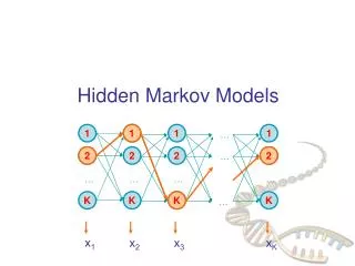
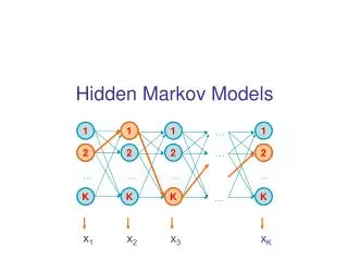
Decoding 1 2 2 1 1 1 1 … 2 2 2 2 … K … … … … x1 K K K K … x2 x3 xK GIVEN x = x1x2……xN We want to find = 1, ……, N, such that P[ x, ] is maximized * = argmax P[ x, ] We can use dynamic programming! Let Vk(i) = max{1,…,i-1} P[x1…xi-1, 1, …, i-1, xi, i = k] = Probability of most likely sequence of states ending at state i = k Lecture 5, Tuesday April 15, 2003
Decoding – main idea Given that for all states k, and for a fixed position i, Vk(i) = max{1,…,i-1} P[x1…xi-1, 1, …, i-1, xi, i = k] What is Vk(i+1)? From definition, Vl(i+1) = max{1,…,i}P[ x1…xi, 1, …, i, xi+1, i+1 = l ] = max{1,…,i}P(xi+1, i+1 = l | x1…xi,1,…, i) P[x1…xi, 1,…, i] = max{1,…,i}P(xi+1, i+1 = l | i ) P[x1…xi-1, 1, …, i-1, xi, i] = maxk P(xi+1, i+1 = l | i = k) max{1,…,i-1}P[x1…xi-1,1,…,i-1, xi,i=k] = el(xi+1)maxk akl Vk(i) Lecture 5, Tuesday April 15, 2003
The Viterbi Algorithm Input: x = x1……xN Initialization: V0(0) = 1 (0 is the imaginary first position) Vk(0) = 0, for all k > 0 Iteration: Vj(i) = ej(xi) maxk akj Vk(i-1) Ptrj(i) = argmaxk akj Vk(i-1) Termination: P(x, *) = maxk Vk(N) Traceback: N* = argmaxk Vk(N) i-1* = Ptri (i) Lecture 5, Tuesday April 15, 2003
The Viterbi Algorithm x1 x2 x3 ………………………………………..xN Similar to “aligning” a set of states to a sequence Time: O(K2N) Space: O(KN) State 1 2 Vj(i) K Lecture 5, Tuesday April 15, 2003
Viterbi Algorithm – a practical detail Underflows are a significant problem P[ x1,…., xi, 1, …, i ] = a01 a12……ai e1(x1)……ei(xi) These numbers become extremely small – underflow Solution: Take the logs of all values Vl(i) = logek(xi) + maxk [ Vk(i-1) + log akl ] Lecture 5, Tuesday April 15, 2003
Example Let x be a sequence with a portion of ~ 1/6 6’s, followed by a portion of ~ ½ 6’s… x = 123456123456…123456626364656…1626364656 Then, it is not hard to show that optimal parse is (exercise): FFF…………………...FLLL………………………...L 6 nucleotides “123456” parsed as F, contribute .956(1/6)6 = 1.610-5 parsed as L, contribute .956(1/2)1(1/10)5 = 0.410-5 “162636” parsed as F, contribute .956(1/6)6 = 1.610-5 parsed as L, contribute .956(1/2)3(1/10)3 = 9.010-5 Lecture 5, Tuesday April 15, 2003
Problem 2: Evaluation Find the likelihood a sequence is generated by the model
Generating a sequence by the model 1 1 1 1 … 2 2 2 2 … … … … … K K K K … Given a HMM, we can generate a sequence of length n as follows: • Start at state 1 according to prob a01 • Emit letter x1 according to prob e1(x1) • Go to state 2 according to prob a12 • … until emitting xn 1 a02 2 2 0 K e2(x1) x1 x2 x3 xn Lecture 5, Tuesday April 15, 2003
A couple of questions Given a sequence x, • What is the probability that x was generated by the model? • Given a position i, what is the most likely state that emitted xi? Example: the dishonest casino Say x = 12341623162616364616234161221341 Most likely path: = FF……F However: marked letters more likely to be L than unmarked letters Lecture 5, Tuesday April 15, 2003
Evaluation We will develop algorithms that allow us to compute: P(x) Probability of x given the model P(xi…xj) Probability of a substring of x given the model P(I = k | x) Probability that the ith state is k, given x A more refined measure of which states x may be in Lecture 5, Tuesday April 15, 2003
The Forward Algorithm We want to calculate P(x) = probability of x, given the HMM Sum over all possible ways of generating x: P(x) = P(x, ) = P(x | ) P() To avoid summing over an exponential number of paths , define fk(i) = P(x1…xi, i = k) (the forward probability) Lecture 5, Tuesday April 15, 2003
The Forward Algorithm – derivation Define the forward probability: fl(i) = P(x1…xi, i = l) =1…i-1P(x1…xi-1, 1,…, i-1, i = l) el(xi) = k 1…i-2 P(x1…xi-1, 1,…, i-2, i-1 = k) akl el(xi) = el(xi) kfk(i-1) akl Lecture 5, Tuesday April 15, 2003
The Forward Algorithm We can compute fk(i) for all k, i, using dynamic programming! Initialization: f0(0) = 1 fk(0) = 0, for all k > 0 Iteration: fl(i) = el(xi) kfk(i-1) akl Termination: P(x) = kfk(N) ak0 Where, ak0 is the probability that the terminating state is k (usually = a0k) Lecture 5, Tuesday April 15, 2003
Relation between Forward and Viterbi VITERBI Initialization: V0(0) = 1 Vk(0) = 0, for all k > 0 Iteration: Vj(i) = ej(xi) maxkVk(i-1) akj Termination: P(x, *) = maxkVk(N) FORWARD Initialization: f0(0) = 1 fk(0) = 0, for all k > 0 Iteration: fl(i) = el(xi) k fk(i-1) akl Termination: P(x) = k fk(N) ak0 Lecture 5, Tuesday April 15, 2003
Motivation for the Backward Algorithm We want to compute P(i = k | x), the probability distribution on the ith position, given x We start by computing P(i = k, x) = P(x1…xi, i = k, xi+1…xN) = P(x1…xi, i = k) P(xi+1…xN | x1…xi, i = k) = P(x1…xi, i = k) P(xi+1…xN | i = k) Forward, fk(i) Backward, bk(i) Lecture 5, Tuesday April 15, 2003
The Backward Algorithm – derivation Define the backward probability: bk(i) = P(xi+1…xN | i = k) = i+1…NP(xi+1,xi+2, …, xN, i+1, …, N | i = k) = l i+1…NP(xi+1,xi+2, …, xN, i+1 = l, i+2, …, N | i = k) = lel(xi+1) akli+1…NP(xi+2, …, xN, i+2, …, N | i+1 = l) = lel(xi+1) akl bl(i+1) Lecture 5, Tuesday April 15, 2003
The Backward Algorithm We can compute bk(i) for all k, i, using dynamic programming Initialization: bk(N) = ak0, for all k Iteration: bk(i) = lel(xi+1) akl bl(i+1) Termination: P(x) = la0l el(x1) bl(1) Lecture 5, Tuesday April 15, 2003
Computational Complexity What is the running time, and space required, for Forward, and Backward? Time: O(K2N) Space: O(KN) Useful implementation technique to avoid underflows Viterbi: sum of logs Forward/Backward: rescaling at each position by multiplying by a constant Lecture 5, Tuesday April 15, 2003
Posterior Decoding We can now calculate fk(i) bk(i) P(i = k | x) = ––––––– P(x) Then, we can ask What is the most likely state at position i of sequence x: Define ^ by Posterior Decoding: ^i = argmaxkP(i = k | x) Lecture 5, Tuesday April 15, 2003
Posterior Decoding For each state, Posterior Decoding gives us a curve of likelihood of state for each position That is sometimes more informative than Viterbi path * Lecture 5, Tuesday April 15, 2003
A+ C+ G+ T+ A- C- G- T- A modeling Example CpG islands in DNA sequences
Example: CpG Islands CpG nucleotides in the genome are frequently methylated (Write CpG not to confuse with CG base pair) C methyl-C T Methylation often suppressed around genes, promoters CpG islands Lecture 5, Tuesday April 15, 2003
Example: CpG Islands In CpG islands, CG is more frequent Other pairs (AA, AG, AT…) have different frequencies Question: Detect CpG islands computationally Lecture 5, Tuesday April 15, 2003
A model of CpG Islands – (1) Architecture A+ C+ G+ T+ CpG Island A- C- G- T- Not CpG Island Lecture 5, Tuesday April 15, 2003

