Download
1 / 37
370 likes | 385 Views
This article examines the decline in inequality in Latin America and explores various factors contributing to this trend. It discusses different measurements of inequality and analyzes the research conducted by Nora Lustig on the topic.

E N D
Inequality in Latin America Joshua Winter | Statistical Computing | April 13, 2018
Background • Latin America is a vital part of the world economy responsible for producing numerous products essential to our everyday lives such as textiles, food and agriculture, and natural resources. • For decades, it has been among the most unequal regions in the world, particularly with regard to income distribution and social welfare. • However, since the late 1990’s inequality has declined based on nearly all available metrics. • Numerous economists and policy makers have attempted to understand why; the vast majority coming up with slightly different conclusions.
perspectives on the decline • Lower inflation rates (Perry, Lopez). • Strong GDP growth, higher tax revenues, and increased foreign direct investment (Tsounta and Osueke). • Increase in the working age population relative to people of non-working age (Addison). • Establishment of conditional (such as sending your child to school) cash transfer programs (Loyka). • Higher participation rate of the poor in the workforce (Addison). • Use of income redistribution programs and industrial privatization (Cornia, Martorano). • Decline in in the informal sector workforce(Acemoglu). • Decline in wage premium for education (Addison). • More stable monetary and fiscal policy collectively as a region (Perry, Lopez).
Measurements of Inequality • Several methods exist, all attempting to compare the distribution of resources by intelligence agents in the market with a maximum entropy random probability distribution. • Atkinson • Gini • Theil • Generalized Entropy Index • Maximum Entropy Random Probability Distribution. • Distribution with largest entropy should be chosen as least informative. • Minimizes the amount of prior information built into the distribution. • Many physical systems tend to move towards maximal entropy configurations over time.
Atkinson Method and Thiel Index • Atkinson: Useful in determining which end of the distribution contributed most to the observed inequality fluctuations (think weighted). Focus is more on social welfare than income • Theil Index: Measure of redundancy, lack of diversity, isolation, segregation, inequality, non-randomness, and compressibility. Calculated as the maximum possible entropy of the data minus the observed entropy.
Gini coefficient • Measure of statistical dispersion used to represent the frequency distribution in terms of the wealth of a country’s residents. • The most commonly used metric for inequality. • U.S. Gini: .469 ( 115th in the world) • Top 3 (.23-.24) : Finland, Faroe Islands, Slovakia • Bottom 3 (.60-.61): South Africa, Micronesia, Haiti • The Gini Coefficient is considered to be one of the most standard methods of calculating inequality. Largely, this is due to it being simpler to understand compared to the Atkinson or Thiel methods.
Gini coefficient Cont’d • Lorenz Curve: Graphical representation of the CDF of the empirical probability distribution of wealth or income. • For small populations, such as islands, it is calculated as half the relative mean absolute difference . • Larger populations, however, use a continuous probability distribution function.
Nora Lustig • Professor of Latin American Economics at Tulane University. • Originally from Argentina. • Worked for Brooking Institution and was founder of the Latin American and Caribbean Economic Association. • Most notably she has collaborated with the World Bank conducting research relating to Latin American inequality. • Key Articles: • ”The decline in inequality in Latin America” • “The rise and fall of income inequality in Latin America” • “Deconstructing the decline of inequality in Latin America”
Overview of research • Conducted beginning in 2009 and finished in 2013. • Time period(s) researched: 1980’s-2010. Although there is some deviation. • Looked at changes over time to in-country variables such as education, government transfers, wage premiums, and institutions. • Done at a macro level focusing on the region as a whole rather than individual countries • Semi-focus on Mexico, Peru, Argentina, and Brazil; four of the largest economies in the region. • Due in part to lack of data on others and that Mexico, Argentina, Brazil, and Peru have seen relatively large declines in terms of inequality in recent years.
Lustig’s analysis • From 2000-2009 the Gini decreased in 13/17 LA countries with comparable data. • Regionally speaking, it decreased from .529-.509. • Stronger labor institutions and greater concern for social issues. • Fall in the wage premium for skilled workers. • Increased educational spending, attainment, educational mobility. • Decline of non-labor income inequality is directly linked to fiscal policy. • The decline in inequality accounted for about a third of the decline of the decline in extreme poverty, the remaining two-thirds were accounted for by economic growth.
Average Level of Inequality 1980-2010 Obs. Year Avg. Gini 1 1980 0.510 2 1986 0.514 3 1992 0.519 4 1998 0.531 5 2002 0.533 6 2008 0.508
Change in inequality 2000-2010 Country Average Annual Change in Gini 2000-2010 (in Percent) 1 Argentina -1.30 2 Bolivia -2.05 3 Brazil -1.03 4 Chile -0.72 5 Costa Rica -0.47 6 Dominican Republic -0.79 7 Ecuador -1.99 8 El Salvador -1.24 9 Guatemala -0.10 10 Honduras 0.61 11 Mexico -1.17 12 Nicaragua -2.64 13 Panama -0.74 14 Paraguay -0.39 15 Peru -0.91 16 Uruguay -0.20 17 Venezuela -1.07 Country Average Annual Change in Gini 200-2010 (in Percent) Length:17 Min. :-2.6400 Class :character 1st Qu.:-1.2400 Mode :character Median :-0.9100 Mean :-0.9529 3rd Qu.:-0.4700 Max. : 0.6100
Average change in inequality vs education Country Gini Secondary Primary Tertiary Average change in Return to Education (P,S,T) 2000-2010 1 Argentina -0.0130 -0.030 0.013 -0.037 -0.018000000 2 Bolivia -0.0205 -0.040 0.020 -0.028 -0.016000000 3 Brazil -0.0103 -0.035 -0.049 -0.022 -0.035333333 4 Chile -0.0072 -0.035 -0.035 0.000 -0.023333333 5 Costa Rica -0.0047 0.022 -0.037 0.015 0.000000000 6 Dominican Republic -0.0079 -0.008 0.008 -0.021 -0.007000000 7 Ecuador -0.0199 -0.002 -0.010 -0.050 -0.020666667 8 El Salvador -0.0124 -0.019 -0.022 0.028 -0.004333333 9 Guatemala -0.0010 0.005 0.020 0.021 0.015333333 10 Mexico -0.0117 0.010 -0.043 -0.025 -0.019333333 11 Nicaragua -0.0264 -0.007 -0.030 -0.017 -0.018000000 12 Panama -0.0074 -0.003 0.020 -0.017 0.000000000 13 Paraguay -0.0039 -0.025 -0.075 -0.010 -0.036666667 14 Peru -0.0091 0.013 -0.060 -0.023 -0.023333333 15 Uruguay -0.0020 0.020 0.018 -0.012 0.008666667 16 Venezuela -0.0107 -0.035 -0.033 0.007 -0.020333333 > summary(gini_and_ed) Country Gini Secondary Primary Tertiary Length:16 Min. :-0.026400 Min. :-0.04000 Min. :-0.07500 Min. :-0.05000 Class :character 1st Qu.:-0.012550 1st Qu.:-0.03125 1st Qu.:-0.03850 1st Qu.:-0.02350 Mode :character Median :-0.009700 Median :-0.00750 Median :-0.02600 Median :-0.01700 Mean :-0.010506 Mean :-0.01056 Mean :-0.01844 Mean :-0.01194 3rd Qu.:-0.006575 3rd Qu.: 0.00625 3rd Qu.: 0.01425 3rd Qu.: 0.00175 Max. :-0.001000 Max. : 0.02200 Max. : 0.02000 Max. : 0.02800 Average change in Return to Education (P,S,T) 2000-2010 Min. :-0.03667 1st Qu.:-0.02133 Median :-0.01800 Mean :-0.01365 3rd Qu.:-0.00325 Max. : 0.01533
Inequality and education overview • Call: • lm(formula = x ~ y) • Y=Average Percent Change Gini • X=Average Percent Change Returns to Education (Tiers are Averaged) • Residuals: • Min 1Q Median 3Q Max • -1.109e-09 -6.983e-10 -1.860e-10 8.702e-10 1.257e-09 • Coefficients: • Estimate Std. Error t value Pr(>|t|) • (Intercept) 1.472e-10 3.917e-10 3.760e-01 0.713 • y 3.000e+00 9.425e-10 3.183e+09 <2e-16 *** • --- • Signif. codes: 0 ‘***’ 0.001 ‘**’ 0.01 ‘*’ 0.05 ‘.’ 0.1 ‘ ’ 1 • Residual standard error: 8.438e-10 on 14 degrees of freedom • Multiple R-squared: 1, Adjusted R-squared: 1 • F-statistic: 1.013e+19 on 1 and 14 DF, p-value: < 2.2e-16
Inequality and Education by tier continued Y=Average Gini Coefficient P=Average Return to Primary Education S=Average Return to Secondary Education T=Average Return to Tertiary Education X=Average Return to Education lm(formula = y ~ P) Residuals: Min 1Q Median 3Q Max -1.59374 -0.20242 0.06702 0.38725 0.96513 Coefficients: Estimate Std. Error t value Pr(>|t|) (Intercept) -1.057581 0.209537 -5.047 0.000178 *** P -0.003773 0.058683 -0.064 0.949645 --- Signif. codes: 0 ‘***’ 0.001 ‘**’ 0.01 ‘*’ 0.05 ‘.’ 0.1 ‘ ’ 1 Residual standard error: 0.7178 on 14 degrees of freedom Multiple R-squared: 0.0002952, Adjusted R-squared: -0.07111 F-statistic: 0.004134 on 1 and 14 DF, p-value: 0.9496 lm(formula = y ~ S) Residuals: Min 1Q Median 3Q Max -1.6257 -0.1598 0.2316 0.3371 0.8078 Coefficients: Estimate Std. Error t value Pr(>|t|) (Intercept) -0.9430 0.1921 -4.910 0.00023 *** S 0.1019 0.0835 1.221 0.24239 --- Signif. codes: 0 ‘***’ 0.001 ‘**’ 0.01 ‘*’ 0.05 ‘.’ 0.1 ‘ ’ 1 Residual standard error: 0.6825 on 14 degrees of freedom Multiple R-squared: 0.09618, Adjusted R-squared: 0.03163 F-statistic: 1.49 on 1 and 14 DF, p-value: 0.2424 lm(formula = y ~ x) Residuals: Min 1Q Median 3Q Max -1.5128 -0.2179 0.1208 0.4117 1.0657 Coefficients: Estimate Std. Error t value Pr(>|t|) (Intercept) -0.8111 0.2317 -3.501 0.00353 ** x 0.1756 0.1179 1.490 0.15853 --- Signif. codes: 0 ‘***’ 0.001 ‘**’ 0.01 ‘*’ 0.05 ‘.’ 0.1 ‘ ’ 1 Residual standard error: 0.667 on 14 degrees of freedom Multiple R-squared: 0.1368, Adjusted R-squared: 0.07514 F-statistic: 2.219 on 1 and 14 DF, p-value: 0.1585 lm(formula = y ~ T) Residuals: Min 1Q Median 3Q Max -1.5100 -0.3229 0.1510 0.3931 0.8516 Coefficients: Estimate Std. Error t value Pr(>|t|) (Intercept) -0.86351 0.18199 -4.745 0.000314 *** T 0.15674 0.07651 2.049 0.059729 . --- Signif. codes: 0 ‘***’ 0.001 ‘**’ 0.01 ‘*’ 0.05 ‘.’ 0.1 ‘ ’ 1 Residual standard error: 0.6297 on 14 degrees of freedom Multiple R-squared: 0.2306, Adjusted R-squared: 0.1757 F-statistic: 4.197 on 1 and 14 DF, p-value: 0.05973
Inequality, Wage Premiums, Supply and Demand of Unskilled workers country gini Wage premium % Change demand unskilled workers % Change supply unskilled workers 1 Argentina -1.30 -2.4 -4.7 2.40 2 Bolivia -2.05 -4.6 -8.7 5.10 3 Brazil -1.03 -3.2 -5.1 4.40 4 Chile -0.72 -1.9 -4.7 1.10 5 Costa Rica -0.47 -2.0 0.1 6.00 6 Dominican Republic -0.79 -0.2 2.8 3.40 7 Ecuador -1.99 -3.2 -6.3 3.40 8 El Salvador -1.24 -0.1 -0.5 -0.03 9 Guatemala -0.10 -1.9 -3.3 2.30 10 Mexico -1.17 -2.8 -6.3 2.20 11 Nicaragua -2.64 -6.9 -14.1 6.60 12 Panama -0.74 -2.6 -4.4 2.40 13 Paraguay -0.39 -5.6 -10.8 6.10 14 Peru -0.91 2.8 -4.6 3.80 15 Uruguay -0.20 -0.9 -1.4 1.10 16 Venezuela -1.07 -4.8 -10.3 4.20 Total % Change supply and demand unskilled workers 1 -2.30 2 -3.60 3 -0.70 4 -3.60 5 6.10 6 6.20 7 -2.90 8 -0.53 9 -1.00 10 -4.10 11 -7.50 12 -2.00 13 -4.70 14 -0.80 15 -0.30 16 -6.10
% Change Inequality vs % change wage premiums of unskilled workers lm(formula = y ~ Wp) Y= % Change Gini Wp= % Change Wage Premium for Unskilled Workers Residuals: Min 1Q Median 3Q Max -1.00351 -0.52726 0.03114 0.36893 1.07265 Coefficients: Estimate Std. Error t value Pr(>|t|) (Intercept) -0.71382 0.23915 -2.985 0.00984 ** Wp 0.13372 0.07053 1.896 0.07881 . --- Residual standard error: 0.6404 on 14 degrees of freedom Multiple R-squared: 0.2043, Adjusted R-squared: 0.1474 F-statistic: 3.594 on 1 and 14 DF, p-value: 0.07881
% Change Inequality vs % change supply of unskilled workers lm(formula = y ~ %Changeinsupplyofunskilledworkers) Residuals: Min 1Q Median 3Q Max -1.2205 -0.4204 0.1040 0.3412 0.9718 Coefficients: Estimate Std. Error t value Pr(>|t|) (Intercept) -0.65765 0.35292 -1.863 0.0835 . Changeinsuppl-0.11543 0.09086 -1.270 0.2246 --- Residual standard error: 0.6798 on 14 degrees of freedom Multiple R-squared: 0.1034,Adjusted R-squared: 0.03933 F-statistic: 1.614 on 1 and 14 DF, p-value: 0.2246
% Change Inequality vs % change Demand of unskilled workers lm(formula = y ~ changeindemandofunskilledworkers) Residuals: Min 1Q Median 3Q Max -0.83836 -0.47380 0.05496 0.32667 1.15478 Coefficients: Estimate Std. Error t value Pr(>|t|) (Intercept) -0.60124 0.23649 -2.542 0.0235 * Changeindema 0.08736 0.03554 2.458 0.0276 * --- Residual standard error: 0.6 on 14 degrees of freedom Multiple R-squared: 0.3014, Adjusted R-squared: 0.2515 F-statistic: 6.041 on 1 and 14 DF, p-value: 0.02762
% Change Inequality vs % Total change supply and Demand of unskilled workers lm(formula = y ~ TotalChangeinsupplyanddemandunskilledworkers) Residuals: Min 1Q Median 3Q Max -1.07324 -0.33598 -0.00802 0.40283 0.92589 Coefficients: Estimate Std. Error t value Pr(>|t|) (Intercept)-0.89478 0.17516 -5.108 0.000159 *** TotalChange 0.08960 0.04395 2.039 0.060836 . --- Residual standard error: 0.6304 on 14 degrees of freedom Multiple R-squared: 0.2289, Adjusted R-squared: 0.1738 F-statistic: 4.156 on 1 and 14 DF, p-value: 0.06084
Inequality vs % change WP, Supply and Demand, total change supply and demand
Issues with Lustig’s analysis • Conclusions are drawn from a limited dataset. • 17 countries rather than 26 • Time frame makes some of her conclusions disputable today given advancements in technology and worldwide GDP growth. • It only looks at 1 specific measure of inequality (Gini) rather than multiple. • Analysis is more qualitative than quantitative and does not include enough regression based analysis. • None of the data is lagged. • Several of her conclusions were found to be false when recreated/ • Trade and other external factors are left out.
Analysis Extension: Research question • Total trade, imports, and exports are a large indicator of how well an economy is performing on the world stage and directly impact GDP. • Highly indicative country’s level of development. • Therefore: Have total trade, total imports, and total exports significantly impacted income inequality in Latin America?
Overview of data • GINI Data from 1998-2013 from UNDP. • Trade data from WITS (World Integrated Trading Solution). • Developed by the World Bank in collaboration with the United Nations Conference on Trade and Development (UNCTAD)) • Started out as totals (in thousands of U.S. dollars) for each variable and country by year and then was converted to logs using R. • Linear-log form: Y =β0 + β1ln(x)+ ℇ
Variables Countries • GINI Coefficient • Country (15 total) • Year (from 1998 to 2013) • Total Trade • Total Imports • Total Exports • Argentina • Bolivia • Brazil • Chile • Columbia • Costa Rica • Dominican Republic • Ecuador • El Salvador • Honduras • Mexico • Nicaragua • Panama • Paraguay • Peru • Uruguay
Gini by country • Inequality Increased: Brazil, Honduras, Costa Rica • Inequality Declined: Argentina, Chile, Colombia, Dominican Republic, Ecuador, El Salvador, Mexico, Nicaragua, Uruguay • Inequality Declined Substantially: Bolivia, Paraguay, Peru, Panama
equations Y (GINI)=β0 + β1lnTotal Trade+ ℇ Y (GINI) =β0 + β1lnTotalExports+ ℇ Y (GINI) =β0 + β1lnTotalImports+ ℇ
Overview of Data: Summary Statistics • Linear-Log Form • Monthly rather than annual (Lustig) • Note: Tables were exported from R to Excel by coding up a function similar to what is below lmOut <- function(res, file="test.csv", ndigit=3, writecsv=T)
Impact of Total Trade on Inequality Y (GINI)=β0 + β1lnTotal Trade+ ℇ
Impact of Total Imports on Inequality Y (GINI) =β0 + β1lnTotalImports+ ℇ
Impact of Total exports on Inequality Y (GINI) =β0 + β1lnTotalExports+ ℇ
Inequality and Trade Statistics • Countries where inequality is not impacted by…. • Total Trade: Brazil • Total Exports: Brazil, Honduras, Nicaragua • Total Imports: Brazil, El Salvador, Nicaragua • Countries where the result is significant and an increase in X increases inequality…. • Total Trade: Costa Rica, Honduras • Total Exports/Total Imports: Costa Rica • Countries where the result is significant and an increase in X decreases inequality…. • Total Trade: Argentina, Bolivia, Chile, Colombia, Dominican Republic, Ecuador, El Salvador, Mexico, Nicaragua Panama, Paraguay, Peru, Uruguay • Total Exports: Argentina, Bolivia, Chile, Colombia, Dominican Republic, Ecuador, El Salvador, Mexico, Panama, Paraguay, Peru, Uruguay • Total imports: Argentina, Bolivia, Chile, Colombia, Dominican Republic, Ecuador, Honduras, Mexico, Panama, Paraguay, Peru, Uruguay
conclusion • 14/15 Latin American countries surveyed trade had a statistically significant impact on inequality. • 12/14 saw inequality decline as trade increased. • 12/15 saw inequality decline as a result of increased total imports and total exports. • Based on the results, trade usually has a significant and positive impact on inequality. • For the most part, it does not matter whether you are importing more or exporting more. The key lies in higher total trade volume. • While authors such as Lustig and Perez focus on government transfers, education, gdp growth, and tax revenue, more research should be done pertaining to trade as an explanation for declining inequality given the results of this study.
Future work • Code up and replicate more of Nora Lustig’s work. • Build out more complicated models with lags. • Add a larger time span and more Latin American countries into the dataset. • Potentially look at types or classifications of goods such as Capital Imports, Capital Exports, Raw Material Exports, Manufactured Goods Exports, Consumer Good Exports, Intermediate Good Exports, Textile Exports. • Optimize fit for each model. • Extension: Code up Gini Coefficient, Atkinson, and Theil Index using R. • Continuous probability distribution functions