Download
1 / 30
370 likes | 855 Views
Anisotropic Aquifers. Tripp Winters . Horizontal Plane Anisotropy. Anisotropy is a common feature in water laid sedimentary deposits (fluvial, clastic lake, deltaic and glacial outwash). Water lain deposits may exhibit anisotropy on the horizontal plain (X,Y if looking down from above)

E N D
Anisotropic Aquifers Tripp Winters
Horizontal Plane Anisotropy • Anisotropy is a common feature in water laid sedimentary deposits (fluvial, clastic lake, deltaic and glacial outwash). • Water lain deposits may exhibit anisotropy on the horizontal plain (X,Y if looking down from above) • Hydraulic conductivity in the direction of flow tends to be greater than that perpendicular to flow, which causes lines of equal drawdown to form ellipses rather than circles.
Vertical Plane Anisotropy • Water laid sedimentary deposits are often “stratified” (have layers of alternating stratum, therefore alternating K’s) • Any layer with a low K will retard vertical flow, but horizontal flow can occur easily through any layer with relatively high K. • When Kh (parallel to the layer) is larger than Kv (perpendicular to layer), the aquifer is said to be “Vertically anisotropic”.
3-D Anistropy • When an aquifer exhibits both vertical and horizontal anisotropy, it has 3-D anisotropy The principal axes are: • Kz: the vertical direction • Kparallel: The direction parallel to stream flow • Kperpendicular: The direction perpendicular to stream flow
Hantush Assumptions • The assumptions listed at the beginning of Chapter 3, with the exception of the third assumption, which is replaced by: The aquifer is homogeneous, anisotropic on the horizontal plane, and of uniform thickness over the area influenced by the pumping test. Some conditions are added: • The flow to the well is in unsteady state; • If the principal directions of anisotropy are known, drawdown data from two piezometers on different rays from the pumped well will be sufficient. If the principal directions of anisotropy are not known, drawdown data must be available from at least three rays of piezometers.
Hantush’s method So, since the shape of equal drawdown is an ellipse in anisotropic aquifers we need to look at the equation of an ellipse in Cartesian coordinates is: where: a= major horizontal axis b= minor horizontal axis c= vertical axis (not used in this case)
Hantush’s Method • If we have one or more piezometers on a ray that froms an angle with the X axis, methods for isotropic aquifers can be applied to obtain values for (KD)e and S/(KD)n. • Consequently, data is needed from more than one ray of piezometers to calculate S and (KD)n (Transmissivity along rays 0 to n originating at the pumped well, plotting all of these KDn’s corresponding to arrays 0 to n will make an ellipse shape).
Hantush’s Method • If is defined as the angle between the first ray of piezometers (n = 1) and the X axis, and as the angle between the nth ray of pizometers and the first ray of piezometers • (KD)n is given by:
Hantush-Thomas’s Method • Method stated that when KDe, as, bs are known the other hydraulic characteristics can be calculated. • Hence, it is not necessary to have values of S/(KD)n, provided that one has sufficient observations to draw the ellipses of equal drawdown.
Assumptions • The Hantush-Thomas method can be applied if the following assumptions and conditions are satisfied: • - The assumptions listed at the beginning of Chapter 3, with the exception of the third assumption, which is replaced by: • The aquifer is homogeneous, anisotropic on the horizontal plane, and of uniform thickness over the area influenced by the pumping test. • The following condition is added: • - The flow to the well is in unsteady state.
Hantush-Thomas’s Method • As stated before, lines of equal drawdown in an isotropic aquifer are circular around the pumped well whereas the lines of equal drawdown in a horizontally anisotropic aquifer form ellipses. The equation of the an ellipses is:
Conditions The assumptions listed at the beginning of Chapter 3, with the exception of the third assumption, which is replaced by: The aquifer is homogeneous, anisotropic on the horizontal plane, and of uniform thickness over the area influenced by the pumping test. • The following conditions are added: -The flow to the well is in an unsteady state; -The aquifer is penetrated by three wells, which are not on one ray. Two of them are pumped in sequence.
Hantush-Thomas’s Method Where: as and bs are the principal axes of the ellipse of equal drawdown s at time Ts (Figure 8.1 C) It can be shown that:
NEUMANN’S EXTENSION OF PAPADOPULOS METHOD • In 1984, Neumann and others showed that the Papadopulos can be used with drawdown data from only three wells so long as two pumping test performed in sequence with two of the wells.
LEAKY AQUIFERS, ANISOTROPIC ON THE HORIZONTAL PLANE • HANTUSH’S METHOD • The flow to a well in a leaky aquifer which is anisotropic on the horizontal plane can be analyzed with a method that is essentially the same as the Hantush method for confined aquifers with anisotropy on the horizontal plane.
LEAKY AQUIFERS, ANISOTROPIC ON THE HORIZONTAL PLANE • The leakage factor, L, is unknown which is given by Hantush in c is constant so equation 8.7 gives the relationship between Ln and L1
LEAKY AQUIFERS, ANISOTROPIC ON THE HORIZONTAL PLANE • The Hantush method can be applied if the following assumptions and conditions are The assumptions listed at the beginning of Chapter 3, with the exception of the first and third assumptions, which are replaced by: • The aquifer is leaky; • The aquifer is homogeneous, anisotropic on the horizontal plane, and of uniform thickness over the area influenced by the pumping test. The following condition is added: • The flow to the well is in an unsteady state.
CONFINED AQUIFERS, ANISOTROPIC ON THE VERTICAL PLANE • WEEKS’S METHOD
LEAKY AQUIFERS, ANISOTROPIC ON THE VERTICAL PLANE • Weeks’s Method
Unconfined aquifers, anisotropic on the vertical plane • Flow to a partially penetrating well in an unconfined aquifer is considered 3-D during the time the delayed watertable response occurs. 3-D flow is affected by anisotropy in the vertical plane. Neumann’s curve fitting method from section 5.1.1 takes this anisotropy into account. • Two other methods can also be used that take vertical plane anisotropy into account when the well is partially penetrating: • Streltsova’s curve-fitting method (Section 10.4.1) • Neuman’s curve-fitting method (Section 10.4.2) • Boulton-Streltsova’s curve-fitting method (Section 11.2.1).