Regional Ocean Modeling System
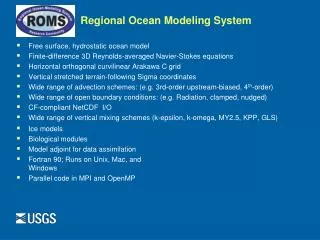
Regional Ocean Modeling System. Free surface, hydrostatic ocean model Finite-difference 3D Reynolds-averaged Navier-Stokes equations Horizontal orthogonal curvilinear Arakawa C grid Vertical stretched terrain-following Sigma coordinates

Regional Ocean Modeling System
E N D
Presentation Transcript
Regional Ocean Modeling System • Free surface, hydrostatic ocean model • Finite-difference 3D Reynolds-averaged Navier-Stokes equations • Horizontal orthogonal curvilinear Arakawa C grid • Vertical stretched terrain-following Sigma coordinates • Wide range of advection schemes: (e.g. 3rd-order upstream-biased, 4th-order) • Wide range of open boundary conditions: (e.g. Radiation, clamped, nudged) • CF-compliant NetCDF I/O • Wide range of vertical mixing schemes (k-epsilon, k-omega, MY2.5, KPP, GLS) • Ice models • Biological modules • Model adjoint for data assimilation • Fortran 90; Runs on Unix, Mac, and Windows • Parallel code in MPI and OpenMP
ROMS wiki - lots of good information https://www.myroms.org/wiki http://www.people.arsc.edu/~kate/ROMS/manual_2012.pdf
Wide Range of realistic Applications 10 km wide island 1,000 km long coastline DongMcWilliamsShchepetkin(2004) 10,000 km wide basin ArangoHaidvogelWilkin(2003) Gruber et al (2004)
W r Dm Wind L H Test Cases • Open channel flow 3) Mixed layer deepening 2) Closed basin, wind-driven circulation 4) Tidal flow around a headland 5) Estuarine circulation http://woodshole.er.usgs.gov/project-pages/sediment-transport/
ROMS Grid - masking - curvature - stretching terrain following coordinates Horizontal Arakawa "C" grid Vertical eta xi
Terrain following transformations (Vtransform + Vstrectching) Vtransform 1 2 https://www.myroms.org/wiki/index.php/Vertical_S-coordinate
Vstretch 1 2 3 4
Equations in Mass Flux form u, v, = Eulerian Velocity ul, vl, = Lagrangian Velocity ust,vst, = Stokes Velocity f = Coriolis parameter φ = Dynamic pressure Hz = Grid cell thickness = Non wave body force = Momentum mixing terms = Non-conservative wave force Continuity xi-direction Momentum Balance
eta-Direction Momentum Balance ACC = Local Acceleration HA = Horizontal Advection VA = Vertical Advection COR = Coriolis Force StCOR = Stokes-Coriolis Force PG = Pressure Gradient HVF = Horizontal Vortex Force BF = Body Force BA+RA+BuSt+SuSt = Breaking Acceleration+ Roller Acceleration+ Bottom Streaming+ Surface Streaming HM = Horizontal Mixing VM = Vertical Mixing Fcurv = Curvilinear terms Description of Terms Kumar, N., Voulgaris, G., Warner, J.C., and M., Olabarrieta (2012). Implementation of a vortex force formalism in a coupled modeling system for inner-shelf and surf-zone applications. Ocean Modelling, 47, 65-95.
Solution techniques- mode splitting Shchepetkin, A. F., and J. C. McWilliams, 2008: Computational kernel algorithms for fine-scale, multi-process, long-time oceanic simulations. In: Handbook of Numerical Analysis: Computational Methods for the Ocean and the Atmosphere, eds. R. Temam & J. Tribbia, Elsevier Science, ISBN-10: 0444518932, ISBN-13: 978-0444518934.
Numerical algorithms Advection schemes - 2nd order centered - 4th order centered - 4th order Akima - 3rd order upwind -MPDATA many choices, see manual for details. ……
How do we select different schemes • c pre-processor definitions (list them in *.h file) • during compilatoin, .F .f90s • compiles f90's into objects • compiles objects to libs • ar the libs to make 1 exe • for coupling, it makes wrf, roms, and/or swan as libs, then pull them together for couplingand only produces one exe COAWSTM.exe
COAWST cpp options • #define ROMS_MODEL if you want to use the ROMS model • #define SWAN_MODEL if you want to use the SWAN model • #define WRF_MODEL if you want to use the WRF model • #define MCT_LIB if you have more than one model selected and you want to couple them • #define UV_KIRBY compute "depth-avg" current based on Hwaveto be sent from the ocn to the wav model for coupling • #define UV_CONST send vel = 0 from the ocn to wave model • #define ZETA_CONST send zeta = 0 from the ocn to wave model • #define ATM2OCN_FLUXES provide consistent fluxes between atm and ocn. • #define MCT_INTERP_WV2AT allows grid interpolation between the wave and atmosphere models • #define MCT_INTERP_OC2AT allows grid interpolation between the ocean and atmosphere models • #define MCT_INTERP_OC2WV allows grid interpolation between the ocean and wave models • #define NESTING allows grid refinement in roms or in swan • #define COARE_TAYLOR_YELLAND wave enhanced roughness • #define COARE_OOST wave enhanced roughness • #define DRENNAN wave enhanced roughness + …………..
ROMS/Include/cppdefs.h See cppdefs for a complete list of ROMS options This list goes on for many many more pages …..
Application example: Sandy 1) roms grid 2) masking 3) bathy 4) child grid 5) 3D: BC's (u,v,temp,salt), init, and climatology 6) 2D: BC's (ubar, vbar, zeta) = tides 7) Surface forcing (heat and momentum fluxes) 8) sandy.h and ocean_sandy.in 9) coawst.bash 10) run it - Handout ends here - More in the online ppt - Classroom tutorial will now follow: Projects/Sandy/create_sandy_application.m
1) Grid generation tools • Seagrid - matlab http://woodshole.er.usgs.gov/operations/ modeling/seagrid/ (needs unsupported netcdf interface) • gridgen - command line http://code.google.com/p/gridgen-c/ • EASYGRID
1) Grid generation tools • COAWST/Tools/mfiles/mtools/wrf2roms _mw.m function wrf2roms_mw(theWRFFile, theROMSFile) Generates a ROMS grid from a WRF grid. • COAWST/Tools/mfiles/mtools/create_roms_xygrid.m intended for simple rectilinear grids • or any other method that you know
1) Grid generation toolssee WRF grid netcdf_load('wrfinput_d01') figure pcolorjw(XLONG,XLAT,double(1-LANDMASK)) hold on % pick 4 corners for roms parent grid % start in lower left and go clockwise corner_lon=[ -82 -82 -62 -62]; corner_lat=[ 28 42 42 28]; plot(corner_lon,corner_lat,'g.','markersize',25) % %pick the number of points in the new roms grid numx=80; numy=64; % % make a matrix of the lons and lats x=[1 numx; 1 numx]; y=[1 1; numynumy]; % z=[corner_lon(1) corner_lon(2) corner_lon(4) corner_lon(3)]; F = TriScatteredInterp(x(:),y(:),z(:)); [X,Y]=meshgrid(1:numx,1:numy); lon=F(X,Y).'; % z=[corner_lat(1) corner_lat(2) corner_lat(4) corner_lat(3)]; F = TriScatteredInterp(x(:),y(:),z(:)); lat=F(X,Y).'; plot(lon,lat,'g+') select 4 corners
1) Grid generation tools % % Call generic grid creation % roms_grid='Sandy_roms_grid.nc'; rho.lat=lat; rho.lon=lon; rho.depth=zeros(size(rho.lon))+100; % for now just make zeros rho.mask=zeros(size(rho.lon)); % for now just make zeros spherical='T'; projection='mercator'; save temp_jcw33.mat eval(['mat2roms_mw(''temp_jcw33.mat'',''',roms_grid,''');'])
2) masking – first base it on WRF F = TriScatteredInterp(double(XLONG(:)),double(XLAT(:)), ... double(1-LANDMASK(:)),'nearest'); roms_mask=F(lon,lat); figure pcolorjw(lon,lat,roms_mask) ncwrite(roms_grid,'mask_rho',roms_mask);
2) Masking – get coastline May also need a coastline, can obtain this here: http://www.ngdc.noaa.gov/mgg/coast/ 45 -84 -60 25 lon=coastline(:,1); lat=coastline(:,2); save coastline.matlonlat
2) Masking use COAWST/Tools/mfiles/mtools/editmask m file (from Rutgers, but I changed it to use native matlabnetcdf) editmask('USeast_grd.nc','coastline.mat')
3) bathymetry many sources Coastal Relief Model ETOPO2 LIDAR
3) bathymetry Interpolate bathy to the variable 'h' located at your grid rho points (lon_rh, lat_rho). load USeast_bathy.mat netcdf_load(roms_grid) h=griddata(h_lon,h_lat,h_USeast,lon_rho,lat_rho); h(isnan(h))=5; figure pcolorjw(lon_rho,lat_rho,h) ncwrite(roms_grid,'h',hnew); - Bathymetry can be smoothed using http://drobilica.irb.hr/~mathieu/Bathymetry/index.html
Grid Parameters Beckman & Haidvogel number (1993) Haney number (1991) should be < 0.2 but can be fine up to ~ 0.4 determined only by smoothing should be < 9 but can be fine up to ~ 16 in some cases determined by smoothing AND vertical coordinate functions If these numbers are too large, you will get large pressure gradient errors and Courant number violations and the model will typically blow up right away
4) Child grid ref_ratio=3; roms_child_grid='Sandy_roms_grid_ref3.nc'; F=coarse2fine('Sandy_roms_grid.nc','Sandy_roms_grid_ref3.nc', ... ref_ratio,Istr,Iend,Jstr,Jend); Gnames={'Sandy_roms_grid.nc','Sandy_roms_grid_ref3.nc'}; [S,G]=contact(Gnames,'Sandy_roms_contact.nc');
4) Child grid Redo Bathymetry: load USeast_bathy.mat netcdf_load(roms_grid) h=griddata(h_lon,h_lat,h_USeast,lon_rho,lat_rho); figure pcolorjw(lon_rho,lat_rho,h) ncwrite(roms_grid,'h',hnew); Redo masking % recompute child mask based on WRF mask netcdf_load('wrfinput_d02'); F = TriScatteredInterp(double(XLONG(:)),double(XLAT(:)), ... double(1-LANDMASK(:)),'nearest'); roms_mask=F(lon_rho,lat_rho); figure pcolorjw(lon_rho,lat_rho,roms_mask)
5) 3D BC's (u,v,temp,salt), init, and clima. Projects/Sandy/roms_master_climatology_sandy.m This works for multiple days. Needs nctoolbox to acess data via thredds server. http://code.google.com/p/nctoolbox/
5) 3D BC's (u,v,temp,salt), init, and clima. % I copied Tools/mfiles/roms_clm/roms_master_climatology_coawst_mw.m % to Projects/Sandy/roms_master_climatology_sandy.m and ran it: roms_master_climatology_sandy % this created three files: % merged_coawst_clm.nc % merged_coawst_bdy.nc % coawst.ini.nc % I renamed those to Sandy_clm.nc, Sandy_bdy.nc, and Sandy_ini.nc. %
5) For child grid need init and clim. • Init for child you can use create_roms_child_init • For child clim you can use create_roms_child_clm
6) 2D: BC's (ubar, vbar, zeta) = tides 1) Get the tidal data at svncheckout https://coawstmodel.sourcerepo.com/coawstmodel/data . 2) edit Tools/mfiles/tides/create_roms_tides
6) 2D: BC's (ubar, vbar, zeta) = tides netcdf_load('Sandy_roms_grid.nc') pcolorjw(lon_rho,lat_rho,squeeze(tide_Eamp(:,:,1))) M2 tidal amplitude
7) Surface forcings (wind stress only)- narr2romsnc.m COAWST/Tools/mfiles/mtools/ narr2romsnc creates netcdf forcing files for ROMS. Many others tools available. Can also use ana_functions.
7) Surface forcings (heat + momentum) create_roms_forcings.m COAWST/Tools/mfiles/mtools/ create_roms_forcings creates netcdf forcing files for ROMS. Many others tools available.
Output sustr temp (surface) It’s that easy. I don’t understand why people have problems.