Download
1 / 33
340 likes | 558 Views
Introduction to Binomial Trees. Chapter 12. Goals of Chapter 12. Introduce the binomial tree model in the one-period case Discuss the risk-neutral valuation relationship Introduce the binomial tree model in the two-period case and the CRR binomial tree model

E N D
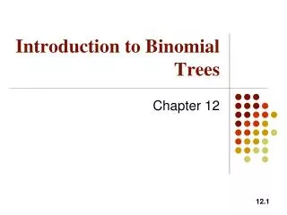
Introduction to Binomial Trees Chapter 12
Goals of Chapter 12 • Introduce the binomial tree model in the one-period case • Discuss the risk-neutral valuation relationship • Introduce the binomial tree model in the two-period case and the CRR binomial tree model • Consider the continuously compounding dividend yield in the binomial tree model
One-Period Binomial Tree Model • The binomial tree model represents possible stock price at any time point based on a discrete-time and discrete-price framework • For a stock price at a time point, a binomial distribution models the stock price movement at the subsequent time point • That is, there are two possible stock prices with assigned probabilities at the next time point • The binomial tree model is a general numerical method for pricing derivatives with various payoffs • The binomial tree model is particularly useful for valuing American options, which do not have analytic option pricing formulae
One-Period Binomial Tree Model = 22 = 20 = 18 • One-period case for the binomial tree model • The stock price is currently $20 • After three months, it will be either $22 or $18 for the upper and lower branches
One-Period Binomial Tree Model = 22 = 1 = 20 = ? = 18 = 0 • Consider a 3-month call option on the stock with a strike price of 21 • Corresponding to the upper and lower movements in the stock price, the payoffs of this call option are = $1 and = $1 • What is the theoretical value of this call today?
One-Period Binomial Tree Model 22D – 1 18D • Consider a portfolio P: long shares short 1 call option • Portfolio P is riskless when 22– 1 = 18, which implies = 0.25 • The value of Portfolio P after 3 months is 22 x 0.25 – 1 = 18 x 0.25 = 4.5
One-Period Binomial Tree Model • Since Portfolio P is riskless, it should earn the risk-free interest rate according to the no-arbitrage argument • If the return of Portfolio P is higher (lower) than the risk-free interest rate Portfolio P is more (less) attractive than other riskless assets Buy (Short) Portfolio P and short (buy) the riskless asset can arbitrage Purchasing (selling) pressure bid up (drive down) the price of Portfolio P, which causes the decline (rise) of the return of Portfolio P • The value of the portfolio today is 4.5= 4.367, where 12% is the risk-free interest rate • The amount of 4.367 should be the cost (or the initial investment) to construct Portfolio P
One-Period Binomial Tree Model • The riskless Portfolio P consists of long 0.25 shares and short 1 call option • The cost to construct Portfolio P equals 0.25 x 20 – • Solve for the theoretical value of this call today to be = 0.633 by equalizing 0.25 x 20 – with 4.367
Generalization of One-Period Binomial Tree Model • Consider any derivative lasting for time T and its payoff is dependent on a stock • Assume that the possible stock price at T are and , where and are constant multiplication factors for the upper and lower branches • and are payoffs of the derivative corresponding to the upper and lower branches
Generalization of One-Period Binomial Tree Model • Construct Portfolio P that longs D shares and shorts 1 derivative. The payoffs of Portfolio P are • Portfolio P is riskless if and thus • Recall that in the prior numerical example, , , , , and , so the solution of for generating a riskless portfolio is 0.25
Generalization of One-Period Binomial Tree Model • Value of Portfolio P at time Tis (or equivalently ) • Value of Portfolio P today is thus • The initial investment (or the cost) for Portfolio P is • Hence • Substituting for in the above equation, we obtain , where
Risk-Neutral Valuation Relationship • Risk-averse, risk-neutral, and risk-loving behaviors • A game of flipping a coin • For risk-averse investors, they accept a risky game if its expected payoff is higher than the payoff of the riskless game by a required amount which can compensate investors for the risk they take • That is, risk-averse investors requires compensation for risk • For different investors, they have different tolerance for risk, i.e., they require different expected payoff to accept the same risky game
Risk-Neutral Valuation Relationship • For risk-neutral investors, they accept a risky game even if its expected payoff equals the payoff of the riskless game • That is, they care about only the levels of the (expected) payoffs • In other words, they require no compensation for risk • For risk-loving investors, they accept a risky game to enjoy the feeling of gamble even if its expected payoff is lower than the payoff of the riskless game • That is, they would like to sacrifice some benefit for entering a risky game
Risk-Neutral Valuation Relationship • In a risk-averse financial market, securities with higher degree of risk need to offer higher expected returns • So, our real world is a risk averse world, i.e., most investors are risk averse and require compensation for the risk they tolerate • In a risk-neutral financial market, the expected returns of all securities equal the risk free rate regardless of their degrees of risk • That is, even for derivatives, their expected returns equal the risk free rate in the risk-neutral world • In a risk-loving financial market, securities with higher degree of risk offer lower expected returns
Risk-Neutral Valuation Relationship • Interpret in as a probability in the risk-neutral world • If the expected return of the stock price is in the real world (a risk averse world), the expected stock price at the end of the period is
Risk-Neutral Valuation Relationship • Comparing with , it is natural to interpret and as probabilities of upward and downward movements in the risk-neutral world • This is because that the expected return of any security in the risk-neutral world is the risk free rate • The formula is consistent with the general rule to price derivatives • Note that in the risk-neutral world, is the expected payoff of a derivative and is the correct discount factor to derive the PV today • The complete version of the general derivative pricing method is that any derivative can be priced as the PV of its expected payoff in the risk-neutral world
Risk-Neutral Valuation Relationship • Risk-neutral valuation relationship (RNVR) • It states that any derivative can be priced with the general derivative pricing rule as if it and its underlying asset were in the risk-neutral world • Since the expected returns of both the derivative and its underlying asset are the risk free rate • The probability of the upward movement in the prices of the underlying asset is • The discount rate for the expected payoff of the derivative is also • When we are evaluating an option on a stock, the expected return on the underlying stock is irrelevant
Risk-Neutral Valuation Relationship = 22 = 1 = 20 = ? = 18 = 0 • Revisit the original numerical examplein the risk-neutral world • Calculate • Calculate the option value according to the RNVR
Two-Period Binomial Tree Model 24.2 • Note the recombined feature can limit the growth of the number of nodes on the binomial tree in a acceptable manner 22 19.8 20 18 16.2 • Values of the parameters of the binomial tree • , , , , , the number of time steps is , and thus the length of each time step is • Hence, the risk-neutral probability
Two-Period Binomial Tree Model node D node B 24.2 3.2 22 2.0257 node E node A 19.8 0 20 1.2823 node C node F 18 16.2 0 0 • For a European call option with the strike price to be 21, perform the backward induction method (逆向歸納法)recursivelyon the binomial tree • Option value at node B: • Option value at node C: • Option value at node A (the initial or root node):
Two-Period Binomial Tree Model node D node B 72 0 60 1.4147 node A node E 50 4.1923 48 4 node C node F 40 32 20 9.4636 • For a European put with and • , , , , , , and • Option value at node B: • Option value at node C: • Option value at node A:
Binomial Tree Model for American Options node D node B 72 0 60 1.4147 node A node E 50 5.0894 48 4 node C node F 40 32 20 12 • For an American put with and • Option value at node B: • Option value at node C: , which is smaller than the exercise value it is optimal to early exercise • Option value at node A:
Delta • Delta () • The formula to calculate in the binomial tree model is on Slide 12.11 • In the binomial tree model, is the number of shares of the stock we should hold for each option shorted in order to create a riskless portfolio • For the one-period example on Slide 12.6, the delta of the call option is • Theoretically speaking, is defined as the ratio of the change in the price of a stock option with respect to the change in the price of the underlying stock, i.e.,
Delta • The delta hedging strategy is a procedure to eliminate the price risk and construct a riskless portfolio for a period of time (introduced in Ch. 17) • The method to decide the value of the delta in the binomial tree model is in effect to perform the delta hedging strategy • Long shares andshort 1 derivative form a portfolio to be • Since we determine such that the portfolio is riskless, it implies that the value of this portfolio is immunized to the change in stock prices, i.e., • Thus, we can solve
Delta node D node B 24.2 3.2 22 2.0257 node E node A 19.8 0 20 1.2823 node C node F 18 16.2 0 0 • The value of varies from node to node (revisit the call option on Slide 12.23) • at node A: • at node B: • at node C:
Delta • Since the value of changes over time, the delta hedging strategy needs rebalances over time • For node A, is decided to be 0.5024 such that the portfolio is riskless during the first period of time • If the stock price rises (falls) to reach node B (C), changes to 0.7273 (0), which means that we need to increase (reduce) the number of shares held to make the portfolio risk free in the second period
CRR Binomial Tree Model • How to determine and • In practice, given any stock price at the time point , and are determined to match the variance of the stock price at the next time point
CRR Binomial Tree Model With and the assumption of and • This method is first proposed by Cox, Ross, and Rubinstein (1979), so this method is also known as the CRR binomial tree model • The validity of the CRR binomial tree model depends on the risk-neutral probability being in [0,1] • In practice, the life of the option is typically partitioned into hundreds time steps • First, ensure the validity of the risk-neutral probability, , which approaches 0.5 if approaches 0 • Second, ensure the convergence to the Black–Scholes model (introduced in Ch. 13)
The Effect of Dividend Yield on Risk-Neutral Probabilities • In the risk-neutral world, the total return from dividends and capital gains is • If the dividend yield is , the return of capital gains in the stock price should be • Hence, • The dividend yield does NOT affect the volatility of the stock price and thus does NOT affect the multiplying factors and • So, and in the CRR model still can be used