Data Structures and Algorithms CSCE 221
Data Structures and Algorithms CSCE 221. Dr. Scott Schaefer. Staff. Instructor Dr. Scott Schaefer HRBB 527B Office Hours: MTWR 9:30am – 10am, F 9am-10am (or by appointment) TA Zain Shamsi HRBB 501C Office Hours: TR noon-2pm Peer Teacher Colton Williams RDMC 111B

Data Structures and Algorithms CSCE 221
E N D
Presentation Transcript
Data Structures and Algorithms CSCE 221 Dr. Scott Schaefer
Staff • Instructor • Dr. Scott Schaefer • HRBB 527B • Office Hours: MTWR 9:30am – 10am, F 9am-10am (or by appointment) • TA • Zain Shamsi • HRBB 501C • Office Hours: TR noon-2pm • Peer Teacher • Colton Williams • RDMC 111B • Office Hours: MW noon-1pm, F noon-2pm
What will you learn? Analysis of Algorithms Stacks, Queues, Deques Vectors, Lists, and Sequences Trees Priority Queues & Heaps Maps, Dictionaries, Hashing Skip Lists Binary Search Trees Sorting and Selection Graphs
Prerequisites • CSCE 121 “Introduction to Program Design and Concepts” or (ENGR 112 “Foundations of Engineering” and CSCE 113 “Intermediate Programming & Design”) • CSCE 222 “Discrete Structures” or MATH 302 “Discrete Mathematics” (either may be taken concurrently with CSCE 221)
More on Assignments • Turn in code/homeworks via CSNET (get an account if you don’t already have one) • Due by 11:59pm on day specified • All programming in C++ • Code, proj file, sln file, and Win32 executable • Make your code readable (comment) • You may discuss concepts, but coding is individual (no “team coding” or web)
Grading • 3% Labs • 12% Homework • 35% Programming Assignments • 10% Quizzes • 20% Midterm • 20% Final
Late Policy • Penalty = m: number of minutes late Percentage Penalty Days Late
Late Policy • Penalty = m: number of minutes late Percentage Penalty Days Late
Late Policy • Penalty = m: number of minutes late Percentage Penalty Days Late
Labs • Several structured labs at the beginning of class with (simple) exercises • Graded on completion • Time to work on homework/projects
Homework Between 5-10 Written/Typed responses Simple coding if any
Programming Assignments 5 throughout the semester Implementation of data structures or algorithms we discusses in class Written portion of the assignment
Quizzes • Approximately 10 throughout the semester • Short answer, small number of questions • Will only be given in class or lab • Must be present to take the quiz
Academic Honesty • Assignments are to be done on your own • May discuss concepts, get help with a persistent bug • Should not copy work, download code, or work together with other students unless specifically stated otherwise • We use a software similarity checker
Class Discussion Board piazza.com/tamu/summer2013/csce221100 Sign up as a student
Asymptotic Analysis 17/36
Running Time • The running time of an algorithm typically grows with the input size. • Average case time is often difficult to determine. • We focus on the worst case running time. • Crucial to applications such as games, finance and robotics • Easier to analyze worst case 5ms 4ms Running Time 3ms best case 2ms 1ms A B C D E F G Input Instance 18/36
Experimental Studies • Write a program implementing the algorithm • Run the program with inputs of varying size and composition • Use a method like clock() to get an accurate measure of the actual running time • Plot the results 19/36
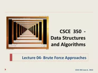
Stop Watch Example 20/36
Limitations of Experiments • It is necessary to implement the algorithm, which may be difficult • Results may not be indicative of the running time on other inputs not included in the experiment. • In order to compare two algorithms, the same hardware and software environments must be used 21/36
Theoretical Analysis • Uses a high-level description of the algorithm instead of an implementation • Characterizes running time as a function of the input size, n. • Takes into account all possible inputs • Allows us to evaluate the speed of an algorithm independent of the hardware/software environment 22/36
Important Functions • Seven functions that often appear in algorithm analysis: • Constant 1 • Logarithmic log n • Linear n • N-Log-N n log n • Quadratic n2 • Cubic n3 • Exponential 2n 23/36
Important Functions • Seven functions that often appear in algorithm analysis: • Constant 1 • Logarithmic log n • Linear n • N-Log-N n log n • Quadratic n2 • Cubic n3 • Exponential 2n 24/36
Why Growth Rate Matters runtime quadruples when problem size doubles 25/36
Comparison of Two Algorithms insertion sort is n2 / 4 merge sort is 2 n lg n sort a million items? insertion sort takes roughly 70 hours while merge sort takes roughly 40 seconds This is a slow machine, but if 100 x as fast then it’s 40 minutes versus less than 0.5 seconds 26/36
Constant Factors • The growth rate is not affected by • constant factors or • lower-order terms • Examples • 102n+105is a linear function • 105n2+ 108nis a quadratic function 27/36
Big-Oh Notation • Given functions f(n) and g(n), we say that f(n) is O(g(n)) if there are positive constantsc and n0 such that f(n)cg(n) for n n0 • Example: 2n+10 is O(n) • 2n+10cn • (c 2) n 10 • n 10/(c 2) • Pick c = 3 and n0 = 10 28/36
Big-Oh Example • Example: the function n2is not O(n) • n2cn • n c • The above inequality cannot be satisfied since c must be a constant 29/36
More Big-Oh Examples 7n-2 7n-2 is O(n) need c > 0 and n0 1 such that 7n-2 c•n for n n0 this is true for c = 7 and n0 = 1 • 3n3 + 20n2 + 5 3n3 + 20n2 + 5 is O(n3) need c > 0 and n0 1 such that 3n3 + 20n2 + 5 c•n3 for n n0 this is true for c = 4 and n0 = 21 • 3 log n + 5 3 log n + 5 is O(log n) need c > 0 and n0 1 such that 3 log n + 5 c•log n for n n0 this is true for c = 8 and n0 = 2 30/36
Big-Oh and Growth Rate • The big-Oh notation gives an upper bound on the growth rate of a function • The statement “f(n) is O(g(n))” means that the growth rate of f(n) is no more than the growth rate of g(n) • We can use the big-Oh notation to rank functions according to their growth rate 31/36
Big-Oh Rules • If is f(n) a polynomial of degree d, then f(n) is O(nd), i.e., • Drop lower-order terms • Drop constant factors • Use the smallest possible class of functions • Say “2n is O(n)” instead of “2n is O(n2)” • Use the simplest expression of the class • Say “3n+5 is O(n)” instead of “3n+5 is O(3n)” 32/36
Computing Prefix Averages • We further illustrate asymptotic analysis with two algorithms for prefix averages • The i-th prefix average of an array X is average of the first (i+ 1) elements of X: A[i]= (X[0] +X[1] +… +X[i])/(i+1) 33/36
Prefix Averages (Quadratic) The following algorithm computes prefix averages in quadratic time by applying the definition AlgorithmprefixAverages1(X, n) Input array X of n integers Output array A of prefix averages of X #operations A new array of n integers n fori 0 ton 1 do n s X[0] n forj 1 toido 1 + 2 + …+ (n 1) s s+X[j] 1 + 2 + …+ (n 1) A[i] s/(i+ 1)n returnA 1 34/36
The running time of prefixAverages1 isO(1 + 2 + …+ n) The sum of the first n integers is n(n+ 1) / 2 Thus, algorithm prefixAverages1 runs in O(n2) time Arithmetic Progression 35/36
Prefix Averages (Linear) The following algorithm computes prefix averages in linear time by keeping a running sum AlgorithmprefixAverages2(X, n) Input array X of n integers Output array A of prefix averages of X #operations A new array of n integers n s 0 1 fori 0 ton 1 do n s s+X[i] n A[i] s/(i+ 1)n returnA 1 Algorithm prefixAverages2 runs in O(n) time 36/36