ECE 576 – Power System Dynamics and Stability

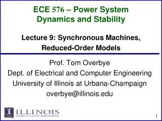
1. ECE 576– Power System Dynamics and Stability Lecture 9: Synchronous Machines, Reduced-Order Models Prof. Tom Overbye Dept. of Electrical and Computer Engineering University of Illinois at Urbana-Champaign overbye@illinois.edu

2. Announcements • Homework 2 is posted on the web; it is due on Thursday Feb 20 • Read Chapter 5 and Appendix A • Read Chapter 6 • A key paper for today's topic is P.V. Kokotovic, and P.W. Sauer, "Integral Manifold as a Tool for Reduced-Order Modeling of Nonlinear Systems: A Synchronous Machine Case Study," IEEE Trans. Circuits and Sys., March 1989 • "Make it as simple as possible but not simpler"

3. Determining d without Saturation • Recalling the relation between d and the stator values • And from 3.215 and 3.216 (in steady-state) • Then use 3.222 and 3.223 to replace

4. Determining d without Saturation • And use 3.219 to eliminate E'd

5. Determining d without Saturation • Which can be rewritten as

6. Determining d without Saturation • Then in terms of the terminal values

7. D-q Reference Frame • Machine voltage and current are “transformed” into the d-q reference frame using the rotor angle,  • Terminal voltage in network (power flow) reference frame are VS = Vt = Vr +jVi

8. A Steady-State Example • Assume a generator is supplying 1.0 pu real power at 0.95 pf lagging into an infinite bus at 1.0 pu voltage through the below network. Generator pu values are Rs=0, Xd=2.1, Xq=2.0, X'd=0.3, X'q=0.5

9. A Steady-State Example, cont. • First determine the current out of the generator from the initial conditions, then the terminal voltage

10. A Steady-State Example, cont. • We can then get the initial angle and initial dq values • Or

11. A Steady-State Example, cont. • The initial state variable are determined by solving with the differential equations equal to zero.

12. PowerWorld Two-Axis Model • Numerous models exist for synchronous machines, some of which we'll cover in-depth. The following is a relatively simple model that represents the field winding and one damper winding; it also includes the generator swing eq. For a salient polemachine, with Xq=X'q, then E'dwould rapidlydecay to zero

13. PowerWorld Solution of 11.10

14. Nonlinear Magnetic Circuits • Nonlinear magnetic models are needed because magnetic materials tend to saturate; that is, increasingly large amounts of current are needed to increase the flux density Linear

15. Saturation

16. Saturation Models • Many different models exist to represent saturation • There is a tradeoff between accuracy and complexity • Book presents the details of fully considering saturation in Section 3.5 • One simple approach is to replace • With

17. Saturation Models • In steady-state this becomes • Hence saturation increases the required Efd to get a desired flux • Saturation is usually modeled using a quadratic function, with the value of Se specified at two points (often at 1.0 flux and 1.2 flux) A and B aredetermined fromthe two data points

18. Saturation Example • If Se = 0.1 when the flux is 1.0 and 0.5 when the flux is 1.2, what are the values of A and B using the

19. Implementing Saturation Models • When implementing saturation models in code, it is important to recognize that the function is meant to be positive, so negative values are not allowed • In large cases one is almost guaranteed to have special cases, sometimes caused by user typos • What to do if Se(1.2) < Se(1.0)? • What to do if Se(1.0) = 0 and Se(1.2) <> 0 • What to do if Se(1.0) = Se(1.2) <> 0 • Exponential saturation models have been used • We'll cover other common saturation approaches in Chapter 5

20. Reduced Order Models • Before going further, we will consider a formal approach to reduce the model complexity • Reduced order models • Idea is to approximate the behavior of fast dynamics without having to explicitly solve the differential equations • Essentially all models have fast dynamics that not explicitly modeled • Goal is a more easily solved model (i.e., a reduced order model) without significant loss in accuracy

21. Manifolds • Hard to precisely define, but "you know one when you see one" • Smooth surfaces • In one dimensions a manifold is a curve without any kinks or self-intersections (line, circle, parabola, but not a figure 8)

22. Two-Dimensional Manifolds Images from book and mathworld.wolfram.com

23. Integral Manifolds Desire is to expressz as an algebraicfunction of x,eliminatingdz/dt Suppose we could find z = h(x)

24. Integral Manifolds Replace z by h(x) Chain rule of differentiation If the initial conditionssatisfy h, so z0 = h(x0)then the reducedequation is exact

25. Integral Manifold Example • Assume two differential equations with z considered "fast" relative to x

26. Integral Manifold Example • For this simple system we can get the exact solution

27. Solve for Equilibrium (Steady-state ) Values

28. Solve for Remaining Constants • Use the initial conditions and derivatives at t=0 to solve for the remaining constants

29. Solve for Remaining Constants

30. Solution Trajectory in x-z Space • Below image shows some of the solution trajectories of this set of equations in the x z space z rapidly decaysto 1.0

31. Candidate Manifold Function • Consider a function of the form z = h(x) = mx + c • We would then have One equation and two unknowns: One solution is m=0, c=1

32. Candidate Manifold Function • With the manifold z = 1 we have an exact solution if z = 1.0 since dz/dt = -10z+10 is always zero • With this approximation then we simplify as This is exact only if z0 = 1.0 Exact solution

33. Linear Function, Full Coupling • Now consider the linear function

34. Linear Function, Full Coupling • Which has an equilibrium point at the origin, eigenvalues l1 = -2.3 (the slow mode) and l2 = -8.7 (the fast mode), and a solution of the form • Using x0 = 10 and z0 = 10, the solution is

35. Solution Trajectory in x-z Space

36. Linear Function, Full Coupling • Same function but change the initial condition to x0= 0 and z0 = 10 • Solving for the constants gives • In general

37. Solution Trajectories in x-z Space

38. Candidate Manifold Function • Trajectories appear to be heading to origin along a single axis • Again consider a candidate manifold functionz = h(x) = mx + c • Again solve for m dx/dt

39. Candidate Manifold Function

40. Candidate Manifold Function • The two solutions correspond to the two modes • The one we've observed is z = -1.3x • The other is z = -7.7x • To observe this mode select x0 = 1and z0 = -7.7 • Zeroing out c1 and c3 is clearly a special case

41. Eliminating the Fast Mode • Going with z = -1.3x we just have the equation • This is a simpler model, with the application determining whether it is too simple

42. Formal Two Time-Scale Analysis • This can be more formalized by introducing a parameter e In the previous example we had e = 0.1

43. Formal Two Time-Scale Analysis • Using the previous process to get an expression for dx/dt we have • For c(e) = 0 Result is complex for larger valuessince system hascomplex eigenvaues

44. Formal Two Time-Scale Analysis • If z is infinitely fast (e = 0) then z = -x, h(e) = -1 • To compute for small euse a power series

45. Formal Two Time-Scale Analysis • Solving for the coefficients

46. Applying to the Previous Example Note the slow mode eigenvalue approximation has changed from -2.3 to -2.2

47. General two-time-scale linear system • To generalize assume Expression for z isthe equilibrium manifold;D must be nonsingular

48. Application to Nonlinear Systems • For machine models this needs to be extended to nonlinear systems In general solution is difficult, but there are special cases similar to the stator transient problem

49. Example

50. Example • Solving we get