Download
1 / 27
270 likes | 372 Views
The Fraction of Ch asteroids in the C complex from SDSS observations. Andrew S. Rivkin JHU/APL. C-complex asteroids. Dominate outer belt, and asteroid belt as a whole Most of the largest asteroids (and at least one dwarf planet!) are classified in this group

E N D
The Fraction of Ch asteroids in the C complex from SDSS observations Andrew S. Rivkin JHU/APL
C-complex asteroids • Dominate outer belt, and asteroid belt as a whole • Most of the largest asteroids (and at least one dwarf planet!) are classified in this group • Associated with carbonaceous chondrites • C class/complex traditionally (if unfortunately) divided into subclasses, including one also named C. • Some with hydrated/hydroxylated minerals, some not. • Absorption band near 3 µm diagnostic for hydrated/hydroxylated minerals
C-complex asteroids • Dominate outer belt, and asteroid belt as a whole • Most of the largest asteroids (and at least one dwarf planet!) are classified in this group • Associated with carbonaceous chondrites • C class/complex traditionally (if unfortunately) divided into subclasses, including one also named C. • Some with hydrated/hydroxylated minerals, some not. • Absorption band near 3 µm diagnostic for hydrated/hydroxylated minerals • Would be useful for all sorts of reasons to at least get a ballpark estimate of what’s out there, hydrated/hydroxylated mineral-wise
Estimation du “ballpark”? Qu'est-ce que c'est? • Does the amount of hydrated material vary greatly among C asteroids? • Some dynamical models would predict a well-mixed asteroid belt w/r/t/ C asteroid types • Are there trends with size? Semi-major axis? • Such trends would (could?) speak to the “ice line” and alteration timescales and processes • Can we use hydrated minerals to trace meteorite types? • Could be used as an independent measure of the bias of the meteorite collection (also, see #1)
The 0.7-µm proxy band • Due to the inconvenience of observing near 3 µm and the limited number of suitable telescope/instrument combinations, “proxy” band desirable • Vilas and Howell have put lots of effort into study and analysis of band near 0.7 µm • Bus/DeMeo Taxa with proxy band: Ch, Cgh called “Ch” in this talk • Bus/DeMeo Taxa without: C, B, Cg, Cb called “C” in this talk ~ ~ Vilas and Sykes (1996)
The 0.7-µm proxy band • This band is correlated with 3- µm band: • Objects with proxy band will also have 3- µm band • Those without have ~50% chance of having 3- µm band • Using proxy band on an individual object could be difficult, but should be hunky-dory for large survey • Luckily, there’s a large survey floating around… Vilas and Sykes (1996)
Target Sample • SDSS Moving Object Catalog 3 • 67637 observations of 43424 known objects • Photometric nights • Filter out sample to most C-like using a* (Ivezic et al.) and limits on colors • 3951 observations of 3102 objects • 1476 with H > 15 (D < ~5 km) • Compare: 405 C-complex objects in SMASS, 193 in S3OS2 (with 85 in common)
Making the call • The presence/absence of the 0.7-µm band can be approximated by looking at the position of the i’ measurement relative to r’ and z’ • Not a perfect measure, but a reasonable start, eh? • Below the line = “Ch” • Above the line = “C” • We’ll punt the error bars for the moment ~ ~ Lines from SMASS survey, points from SDSS
Nuances to keep in mind • Can’t just look for BD>0 • Half of objects on continuum will look like BD>0 • Biased s.t. Ch too high • Can’t just look for BD > 1σ • Now potentially biased against Ch • Can’t exclude 1σ > BD > 0 • Throw out too many objects • Also probably still biased ~ ~ Lines from SMASS survey, points from SDSS
Nuances to keep in mind • Can’t just look for BD>0 • Half of objects on continuum will look like BD>0 • Biased s.t. Ch too high • Can’t just look for BD > 1σ • Now potentially biased against Ch • Can’t exclude 1σ > BD > 0 • Throw out too many objects • Also probably still biased ~ ~ Lines from SMASS survey, points from SDSS
Two (independent, I think) approaches to the problem • Do chi-sq comparison of a spectrum to Bus/Tholen class averages • Use distribution of band depths to estimate relative contributions of populations
“Color Matching” • Compare g’r’i’z’ colors to convolved SMASS spectra • Assign to closest class (B/C/Cb/Cg/Ch/Cgh), minimizing square of errors • Test on SMASS/S3OS2 overlap with SDSS, recovered correct Ch fraction within uncertainty • However, while group values look good, individual values may give wrong results ~
“Histogram Symmetry” • Measure band depth distribution • Assume C asteroids have BD=0, symmetrical scatter around • Ch asteroids are excess after C asteroid population removed • Variations from full-up two-Gaussian fits to simply comparing number of objects with BD > and < 0. ~ ~ ~
What do these Gaussians mean? • Interpretation A: • There’s a fixed(ish) band depth for the 0.7-µm band, scatter is observational • But we do see different depths in meteorites • Interpretation B: • There’s a distribution of band depths in the real material • That suggests error bars all work themselves out • Interpretation C: • This is overthinking a plate of beans
How about results, not in an unreadable table? ~ Ch fraction, Belt as a whole: • Chi sq: 0.30 • Symmetry: 0.16 • Average 0.23 +/- 0.08 For comparison, SMASS + S3OS2 has Ch fraction of ~0.38 +/- 0.02 Chi sq. suggests C complex is • 38% B class • 13% C class • 18% Cb class But, you know, don’t go crazy with that. • 19% Ch class • 10% Cgh class
…and those Gaussians? • For belt as a whole, sum of gaussian with BD=0 and one with BD ~3-4%, both with scatter ~2% . • Other subsets give similar best-fit band depths for Ch gaussian • This is, admittedly suprisingly, consistent with what’s seen in meteorites • Still might be overthinking it, though. ~
…and those Gaussians? • For belt as a whole, sum of gaussian with BD=0 and one with BD ~3-4%, both with scatter ~2% . • Other subsets give similar best-fit band depths for Ch gaussian • This is, admittedly suprisingly, consistent with what’s seen in meteorites • Still might be overthinking it, though. ~ Cloutis et al., (in press/on the web)
…and those Gaussians? • For belt as a whole, sum of gaussian with BD=0 and one with BD ~3-4%, both with scatter ~2% . • Other subsets give similar best-fit band depths for Ch gaussian • This is, admittedly suprisingly, consistent with what’s seen in meteorites • Still might be overthinking it, though. ~
Trends vs. semi-major axis • Divided belt into inner, outer, middle • Mid-belt has higher Ch fraction, as seen in other work • Outer belt has lowest fraction • Two approaches show different size of variation ~
Trends vs. H magnitude • Symmetry approach sensitive to a, so split that out • General decline in Ch fraction with size seen in earlier work • SDSS data shows (slight?) rise with H > ~12.5 • Chi-sq more well-behaved than symmetry
Trends vs. H magnitude • Symmetry approach sensitive to a, so split that out • General decline in Ch fraction with size seen in earlier work • SDSS data shows (slight?) rise with H > ~12.5 • Chi-sq more well-behaved than symmetry
NEO Implications/Speculation • SMASS Ch/Cgh NEO fraction 1/23 • Mars-crossers 3/10 • Ch/Cgh fraction of NEOs < 1/3 that of Ch fraction of similar-sized MBA • Marchi et al., Delbó et al. suggest orbital evolution low-q orbits destruction of 0.7-µm band • If so, estimate this happens to > 2/3 of NEOs? ~
Dynamical Families • Bus and Binzel (2002) found asteroid families to be homogeneous spectrally • Two C-complex families appear in SDSS sample in large numbers: Themis and Hygiea • Both approaches agree: fewer Ch objects than general population • Approach 2 consistent with Ch fraction ≈ 0
3-µm Implications/Speculation(the original point of this exercise) • Basically all C-complex objects with 0.7-µm band have a 3-µm band • Roughly half of C-complex objects without a 0.7-µm band also have a 3-µm band • So hydrated fraction ≈ Ch +0.5 × C • With overall Ch fraction ~ 0.25 and C fraction ~ 0.75, hydrated fraction ≈ 60-65% • CM ~38% of carbonaceous chondrite falls • Also note smallest fraction of objects has Ch more like 0.3 than 0.25 • Hydrated CC fall fraction ~60?% (but hard to really say) ~ ~ ~
Conclusions • Fraction of “Ch-like” ( ) asteroids ≈ 23 ± 8% of C complex • Themis and Hygiea families have fewer asteroids than the background population • The middle asteroid belt has a higher fraction than the inner or outer belts • The fraction reaches an apparent minimum near H ≈ 12, and either remains steady or slowly increases at smaller sizes ~ ~ ~ ~ Ch Ch Ch Ch