Download
1 / 17
170 likes | 190 Views
Eddy activity in the California Current System:. patterns and variability of the potential to kinetic energy conversion, underlying processes. C omparison with the Humboldt system. X. Capet, J. McWilliams, F. Colas ROMS meeting 2007, Los Angeles.

E N D
Eddy activity in the California Current System: patterns and variability of the potential to kinetic energy conversion, underlying processes. Comparison with the Humboldt system X. Capet, J. McWilliams, F. Colas ROMS meeting 2007, Los Angeles
Potential to eddy kinetic energy conversion term: <w'b'> <.> is some appropriate averaging operator. Unless otherwise stated it is a long term (10 years) time average with the seasonal cycle removed. An important quantity !!! 2 ways to compute <w'b'> from model fields. or (2) (1) and then multiply by b Both are roughly equivalent after all (ie there are no bugs in computation of w from (1). Forget my abstract !!!
Configurations: more idealized more realistic 5 ICC grids at various horizontal resolutions (12km, 6km, 3km, 1.5km, 750m). 720 x 720 km. 40 vertical levels, flat bottom, straight coastline. Boundary conditions are provided from 12km idealized USWC outputs (5 days averages). Atmospheric forcing spatially smooth and fixed in time (July COADS climatology) USWC 5km resolution, 32 levels with realistic bathymetry and coastline. Climatological forcings (QuikSCAT + COADS heat and freshwater fluxes). BCs from SODA climatology. Offline coupling: boundary conditions updated every 5 days.
EKE patterns in the CCS ROMS USWC 5km Altimetry Clear offshore EKE maximum along California, ie., away from the unstable coastal jet region.
Explanation for the offshore maximum ? <w'b'> patterns in the CCS -400 -200 0 cross-shore distance [km] • Offshore propagation of eddy activity with inverse cascade • offshore EKE sources (already in Marchesiello et al,2003) annual mean <w'b'> averaged from 0 to 200m The nearshore does not stand out in terms of energy conversion. same as left panel longshore averaged between 34.5 and 41.5o N
<w'b'> patterns in the CCS summer spring fall winter -400 -200 0 -400 -200 0 cross-shore distance [km] cross-shore distance [km] There is also offshore propagation of the EKE sources (<w'b'>), which further highlights the intricate relationship between (seasonal) mean circulation and eddy activity. depth-integrated (0 to 200m) and longshore-averaged (34.5 to 41.5o N) <w'b'>
Alongshore-averaged structure of <w'b'> Annual mean longshore-averaged (34.5 to 41.5o N) <w'b'> x-z section of <w'b'> reveals three types of processes that release available potential energy: • Baroclinic instability of the coastal jet • Baroclinic instability of the CCS • Boundary layer (BL) buoyancy flux (BL restratification tendency)
Near surface <w'b'> : ageostrophic secondary circulations associated with submesoscale fronts buoyancy and associated w in a CCS 750m horizontal resolution solution. w is downward on the cold side, upward on the warm side b W x [km] Submesoscale is not resolved at 5km horizontal resolution. However the same mechanism of restratification by ASCs around fronts is present. Because of larger dissipation/diffusion, front intensification is much reduced and so are wrms and <w'b'>
Near surface <w'b'> : Mixed-layer baroclinic instability ualong u'along uacross u'across w w' Submesoscale instability growth is overwhelmingly due to w'b'. Its length scale is coherent with a “mixed layer deformation radius (Boccaletti et al, 2007). In the CCS submesoscale instability starts showing up around 2.5km horizontal resolution.
Near surface <w'b'> spatial/temporal modulations. <w'b'> averaged from 0 to 50m Signal tends to follow the offshore propagation of the mesoscale (the mesoscale strain is important and so is the mean position of the density front) spring summer vertical vorticity fall winter max and widespread in winter when air-sea fluxes are least stabilizing (or even destabilizing in southern part of the domain) and hbl is deepest (consistent with Fox-Kemper et al (2007), ie., a restratification by secondary circulations scaling as h2bl)
Near surface <w'b'> : where does it go ? Ten-fold increase of near surface <w'b'> between 10 and 1km horizontal resolution. However eddy kinetic energy itself is only moderately affected because the injection takes place in the submesoscale range, ie., within or close to the dissipation range. At resolution around 2-3km a forward cascade of KE shows up to connect the KE source (<w'b'> at submesoscale) and the sink (dissipation at somewhat higher wavenumber). eke injection eke dissipation dx=750m cascade dx=1.5km dx=3km 600km 60km 6km
EKE patterns in the Humboldt system Altimetry ROMS 5km ROMS patterns ok although 20 to 30% overestimate. Offshore EKE maximum as in California, ie., away from the unstable coastal jet region.
<w'b'> patterns in the Humboldt Current System annual mean <w'b'> averaged from 0 to 200m Clear maximum at the coast, ie., baroclinic instability of the coastal jet. Offshore patches of positive <w'b'> consistent with regions of max EKE EKE ROMS 5km
Coastal jet instability in the Humboldt versus CCS Annual mean longshore-averaged (34.5 to 41.5o N) <w'b'> Annual mean longshore-averaged (-32 to -26o N) <w'b'> Humboldt CCS Annual mean longshore velocity (with minus sign) Annual mean longshore velocity The vertical shear is stronger and extends deeper in the Humboldt.
Conclusions: Potential to kinetic energy conversion term was computed for the California and Humboldt systems. Time scales for replenishment of upper ocean (say, 0 to 500m) EKE deduced from <w'b'> are less than 100 days, ie., <w'b'> is a key term in the EKE budget (and <w'b'> distribution does correlate with that of the EKE). Several processes interacting with each other explain the <w'b'>: baroclinic instability of the coastal jet, the offshore mean currents and ageostrophic circulations near fronts (possibly related to submesoscale instabilities). Important differences between California and Humboldt a priori related to the velocity structure of the coastal jet. Sorry for not being with you. Enjoy the wine for me !!
A ROMS meeting in Brazil (eg., Arraial de Cabo, 2 hours drive from Rio) ?? US citizens may need a visa !!!