Download
1 / 54
540 likes | 725 Views
Modelling and Identification of dynamical gene interactions. Ronald Westra , Ralf Peeters Systems Theory Group Department of Mathematics Maastricht University The Netherlands westra@math.unimaas.nl. Themes in this Presentation How deterministic is gene regulation?

E N D
Modelling and Identification of dynamical gene interactions Ronald Westra, Ralf Peeters Systems Theory Group Department of Mathematics Maastricht University The Netherlands westra@math.unimaas.nl.
Themes in this Presentation • How deterministic is gene regulation? • How can we model gene regulation? • How can we reconstruct a gene regulatory network from empirical data ?
1. How deterministic is gene regulation? Main concepts: Genetic Pathway and Gene Regulatory Network
What defines the concepts of agenetic pathwayand agene regulatory networkand how is it reconstructedfrom empirical data ?
G1 G2 G6 G3 G4 G5 Genetic pathway as astatic and fixed model
G1 G2 G6 G3 G4 G5 Experimental method:gene knock-out
How deterministic is gene regulation? Stochastic Gene Expression in a Single Cell M. B. Elowitz, A. J. Levine, E. D. Siggia, P. S. Swain ScienceVol 297 16 August 2002
A B
Conclusions from this experiment Elowitz et al. conclude that gene regulation is remarkably deterministic under varying empirical conditions, and does not depend on particular microscopic details of the genes or agents involved. This effect is particularly strong for high transcription rates. These insights reveal the deterministic nature of the microscopic behavior, and justify to model the macroscopic system as the average over the entire ensemble of stochastic fluctuations of the gene expressions and agent densities.
G1 G2 G6 G3 G4 G5 Implicit modeling: Model only the relations between the genes
Implicit linear model Linear relation between gene expressions Ngene expression profiles : m-dimensional input vectoru(t) : mexternal stimuli p-dimensional output vectory(t) Matrices CandDdefine the selections of expressions and inputs that are experimentally observed
Implicit linear model The matrix A = (aij) - aijdenotes the coupling between geneiand genej: aij > 0 stimulating, aij < 0 inhibiting, aij = 0 : no coupling Diagonal termsaiidenote the auto-relaxation of isolated and expressed genei
G1 G2 G6 G3 G4 coupling from gene 5 to gene 6 is a(5,6) G5 Relation between connectivity matrix A and the genetic pathway of the system
Explicit modeling of gene-gene Interactions In reality genes interact only with agents (RNA, proteins, abiotic molecules) and not directly with other genes Agents engage in complex interactions causing secondary processes and possibly new agents This gives rise to complex, non-linear dynamics
An example of a mathematical model based on some stoichiometric equations using the law of mass actions Here we propose a deterministic approach based on averaging over the ensemble of possible configurations of genes and agents, partly based on the observed reproducibillity by Elowitz et al.
In this model we distinguish between three primary processes for gene-agent interactions: • stimulation • inhibition • transcription • and further allow for secondary processes between agents.
then-vectorxdenotes then gene expressions, them-vectoradenotes the densities of the agents involved.
x: n gene expressions a: magents
(a)denotes the effect of secondary interactions between agents
EXAMPLE Autocatalytic synthesis AgentAicatalyzes its own synthesis:
Complex nonlinear dynamics observed in all dimensionsxanda – including multiple stable equilibria.
Conclusions on modelling More realistic modelling involving nonlinearity and explicit interactions between genes and operons (RNA, proteins, abiotic)exhibits multiple stable equilibriain terms of gene expressions xand agent denisties a
Linear Implicit Model the matricesAandBare unknown u(t)is known andy(t)is observed x(t)is unknown and acts as state space variable
Identification of the linear implicit model the matricesAandBare highly sparse: Most genes interact only with a few other genes or external agents i.e. mostaijandbijare zero.
Challenge for identifying the linear implicit model Estimate the unknown matricesAandBfrom a finite number – M – of samples on times{t1, t2, .., tM}of observations ofinputsuand observationsy: {(u(t1), y(t1)), (u(t2), y(t2)), .., (u(tM), y(tM))}
Notice: • the problem is linear in the unknown parametersAandB • the problem is under-determined as normallyM<<N • the matricesAandBare highly sparse
L2-regression? • This approach minimizes the integral squared error between observed and model values. • This approach would distribute the small scale of the interaction (the sparsity) over all coefficients of the matricesAandB • Hence: this approach would reconstruct small coupling coefficients between all genes – total connectivity with small values and no zeros
L1- or robustregression • This approach minimizes the integral absolute error between observed and model values. • This approach results in generating the maximum amount of exact zeros in the matricesAandB • Hence: this approach reconstructs sparse coupling matrices, in which genes interact with only a few other genes • It is most efficiently implemented with dual linear programming method (dual simplex).
L1-regression Example:Partial dual L1-minimization (Peeters,Westra, MTNS 2004) Involves a number of unobserved genesx in the state space Efficient in terms of CPU-time and number of errors : Mrequired log N
The L1-reconstruction ultimately yields the connectivity matrix Aof the linear implicit model hence the genetic pathway of the gene regulatory system.
Reconstruction of the genetic pathway with partial L1-minimization for the nonlinear explicit model What would the application of this approach yield for directapplication for the explicit nonlinear model discussed before?
Reconstruction with L1-minimization From the explicit nonlinear model one obtains series: {(x(t1), a(t1)), (x(t2), a(t2)), .., (x(tM), a(tM))} For the L1-approach only the terms: {x(t1), x(t2), .., x(tM)} are required.
Conclusions from applying the L1-approach to the nonlinear explicit model 1. The reconstructed connectivity matrix - hence the genetic pathway - differs among different stable equilibria 2. In practical situations to each stable equilibrium there belongs one unique connectivity matrix - hence one unique genetic pathway