Download

1 / 37
370 likes | 476 Views
Linkage in Selected Samples. Boulder Methodology Workshop 2003 Michael C. Neale Virginia Institute for Psychiatric & Behavioral Genetics. Basic Genetic Model. Pihat = p(IBD=2) + .5 p(IBD=1). 1. 1. 1. 1. 1. 1. 1. Pihat. E1. F1. Q1. Q2. F2. E2. e. f. q. q. f. e. P1. P2.

E N D
Linkage in Selected Samples Boulder Methodology Workshop 2003 Michael C. Neale Virginia Institute for Psychiatric & Behavioral Genetics
Basic Genetic Model Pihat = p(IBD=2) + .5 p(IBD=1) 1 1 1 1 1 1 1 Pihat E1 F1 Q1 Q2 F2 E2 e f q q f e P1 P2 Q: QTL Additive Genetic F: Family Environment E: Random Environment3 estimated parameters: q, f and e Every sibship may have different model P P
Mixture distribution model Each sib pair i has different set of WEIGHTS rQ=.0 rQ=1 rQ=.5 weightj x Likelihood under model j p(IBD=2) x P(LDL1 & LDL2 | rQ = 1 ) p(IBD=1) x P(LDL1 & LDL2 | rQ = .5 ) p(IBD=0) x P(LDL1 & LDL2 | rQ = 0 ) Total likelihood is sum of weighted likelihoods
QTL's are factors • Multiple QTL models possible, at different places on genome • A big QTL will introduce non-normality • Introduce mixture of means as well as covariances (27ish component mixture) • Mixture distribution gets nasty for large sibships
Biometrical Genetic Model Genotype means 0 AA m + a -a +a d Aa m + d aa m – a Courtesy Pak Sham, Boulder 2003
Mixture of Normal Distributions :aa :Aa :AA Equal variances, Different means and different proportions
Implementing the Model • Estimate QTL allele frequency p • Estimate distance between homozygotes 2a • Compute QTL additive genetic variance as • 2pq[a+d(q-p)]2 • Compute likelihood conditional on • IBD status • QTL allele configuration of sib pair
27 Component Mixture Sib1 AA Aa aa Sib 2 AA Aa aa
19 Possible Component Mixture Sib1 AA Aa aa Sib 2 AA Aa aa
Results of QTL Simulation 3 Component vs 19 Component 3 Component 19 Component Parameter True Q 0.4 0.414 0.395 A 0.08 0.02 0.02 E 0.6 0.56 0.58 Test Q=0 (Chisq) --- 13.98 15.88 200 simulations of 600 sib pairs each GASP http://www.nhgri.nih.gov/DIR/IDRB/GASP/
Information in selected samples Concordant or discordant sib pairs • Deviation of pihat from .5 • Concordant high pairs > .5 • Concordant low pairs > .5 • Discordant pairs < .5 • How come?
Pihat deviates > .5 in ASP Larger proportion of IBD=2 pairs t IBD=2 Sib 2 IBD=1 IBD=0 t Sib 1
Pihat deviates <.5 in DSP’s Larger proportion of IBD=0 pairs t IBD=2 Sib 2 IBD=1 IBD=0 t Sib 1
Sibship NCP 1.6 1.4 1.2 1 0.8 0.6 0.4 0.2 0 4 3 2 1 -4 0 -3 Sib 2 trait -1 -2 -1 -2 0 1 -3 2 Sib 1 trait 3 -4 4 Sibship informativeness : sib pairs Courtesy Shaun Purcell, Boulder Workshop 03/03
Sibship NCP Sibship NCP 2 2 1.5 1.5 1 1 0.5 0.5 0 4 0 Sibship NCP 3 2 4 1 2 3 -4 0 -3 2 Sib 2 trait -1 -2 1.5 1 -1 -2 0 -4 0 1 1 -3 -3 2 Sib 1 trait Sib 2 trait -2 -1 3 -4 -1 0.5 4 -2 0 1 -3 2 0 Sib 1 trait 3 -4 4 4 3 2 1 -4 0 -3 Sib 2 trait -1 -2 -1 -2 0 1 -3 2 Sib 1 trait 3 -4 4 Sibship informativeness : sib pairs dominance rare recessive unequal allele frequencies Courtesy Shaun Purcell, Boulder Workshop 03/03
Two sources of information Forrest & Feingold 2000 • Phenotypic similarity • IBD 2 > IBD 1 > IBD 0 • Even present in selected samples • Deviation of pihat from .5 • Concordant high pairs > .5 • Concordant low pairs > .5 • Discordant pairs < .5 • These sources are independent
Implementing F&F • Simplest form test mean pihat = .5 • Predict amount of pihat deviation • Expected pihat for region of sib pair scores • Expected pihat for observed scores • Use multiple groups in Mx
Predicting Expected Pihat deviation t IBD=2 Sib 2 + IBD=1 IBD=0 t Sib 1
Expected Pihats: Theory • IBD probability conditional on phenotypic scores x1,x2 • E(pihat) = p(IBD=2|(x1,x2))+p(IBD=1|(x1,x2)) • p(IBD=2|(x1,x2)) = Normal pdf: NIBD=2(x1,x2) p(IBD=2 |(x1,x2))+2p(IBD=1 |(x1,x2))+p(IBD=0 |(x1,x2))
Expected Pihats • Compute Expected Pihats with pdfnor • \pdfnor(X_M_C) • Observed scores X (row vector 1 x nvar) • Means M (row vector) • Covariance matrix C (nvar x nvar)
How to measure covariance? t IBD=2 + IBD=1 IBD=0 t
Ascertainment • Critical to many QTL analyses • Deliberate • Study design • Accidental • Volunteer bias • Subjects dying
Likelihood approach Advantages & Disadvantages • Usual nice properties of ML remain • Flexible • Simple principle • Consideration of possible outcomes • Re-normalization • May be difficult to compute
Example: Two Coin Toss 3 outcomes Frequency 2.5 2 1.5 1 0.5 0 HH HT/TH TT Outcome Probability i = freq i / sum (freqs)
Example: Two Coin Toss 3 outcomes Frequency 2.5 2 1.5 1 0.5 0 HH HT/TH TT Outcome Probability i = freq i / sum (freqs)
Non-random ascertainment Example • Probability of observing TT globally • 1 outcome from 4 = 1/4 • Probability of observing TT if HH is not ascertained • 1 outcome from 3 = 1/3 • or 1/4 divided by ‘Ascertainment Correction' of 3/4 = 1/3
Correcting for ascertainment Univariate case; only subjects > t ascertained N t 0.5 0.4 0.3 G 0.2 likelihood 0.1 0 -4 -3 -2 -1 0 1 2 3 4 : xi
Ascertainment Correction • Be / All you can be N(x) Itx N(x) dx
Affected Sib Pairs 4 4 Itx ItyN(x,y) dy dx + + + 1 0 + + + + + ty + + + + + + + + + + + + + + + + + + + + + + + + + tx 0 1
Selecting on sib 1 4 4 4 Ity I-4 N(x,y) dx dy Ity N(y) dy = + + + 1 0 + + + + + ty + + + + + + + Twin 1 + + + + + + + + + + + + + + + + + + tx Twin 2 0 1
Correcting for ascertainment Dividing by the realm of possibilities • Without ascertainment, we compute • With ascertainment, the correction is pdf, N(:ij,Gij), at observed value xi divided by: I-4 N(:ij,Gij) dx = 1 4 4 It N(:ij,Gij) dx < 1
4 4 Itx ItyN(x,y) dy dx Ascertainment Corrections for Sib Pairs ASP ++ 4 ItxItyN(x,y) dy dx DSP +- -4 ItxItyN(x,y) dy dx CUSP +- -4 -4
Weighted likelihood • Correction not always necessary • ML MCAR/MAR • Prediction of missingness • Correct through weight formula • Use Mx’s \mnor(C_M_U_L_T) • Cov matrix C • Means M • Upper Threshold U • Lower Threshold L • Type T • 0 – below threshold U • 1 – above threshold L • 2 – between threshold • 3 – -infinity to + infinity (ignore)
Normal Theory Likelihood Function For raw data in Mx m ln Li=filn [ 3 wjg(xi,:ij,Gij)] j=1 xi- vector of observed scores onn subjects :ij - vector of predicted means Gij - matrix of predicted covariances - functions of parameters
Correcting for ascertainment Linkage studies • Multivariate selection: multiple integrals • double integral for ASP • four double integrals for EDAC • Use (or extend) weight formula • Precompute in a calculation group • unless they vary by subject
Null Model 50% heritability No QTL Used to generate null distribution .05 empirical significance level at approximately 91 Chi-square QTL Simulations 37.5% heritability 12.5% QTL Mx: 879 significant at nominal .05 p-value Merlin: 556 significant at nominal .05 p-value Some apparent increase in power Initial Results of Simulations
Quantifying QTL variation in selected samples can be done It ain’t easy Can provide more power Could be extended for analysis of correlated traits Conclusion