Download
1 / 14
140 likes | 226 Views
Two Variables. Covariance and Correlation. y. II I III IV. x. When you first encountered the coordinate system used for graphs, you may recall talking about the first quadrant, second quadrant and so as shown in the graph. . y.

E N D
Two Variables Covariance and Correlation
y II I III IV x When you first encountered the coordinate system used for graphs, you may recall talking about the first quadrant, second quadrant and so as shown in the graph.
y II I III IV II I III IV x Later, we might break up what was really the first quadrant into another four quadrants. Please be on the look-out for this.
Overview Sometimes we want to study two variables together. Let’s think about an example about the number of commercials run (variable) during the weekend for a store and the sales volume (variable). Presumably sales volume responds to the number of commercials. Sales volume is the response variable and the number of commercials is the explanatory variable. On the next screen I have a scatter plot of the data. Notice I put the response variable on the vertical, or y, axis. Also notice that I put in lines where the mean of the x and y variables are located. I also put in roman numerals to represent quadrants that I will refer to later.
II x = 3 I y =51 III IV
Thought experiment Imagine we are all in a room together. Say I ask you to turn around, but keep your eyes open. Then I sneak over to the light switch and flip the switch. (by the way, how do you catch a unique bird? U nique up on it!) Now, since the lights were on when we started, let’s say a flip is me turning the switch to off and back to on. So with each flip the lights go off once, but come back on. How many times would the lights go off if I flip the switch 4 times? The lights would go out 4 times! Wouldn’t it be wild it the number of commercials was like me at the switch flipping and the sales were like the lights going going off. We could get sales to be exactly like what we want.
The covariance and correlation measures are designed to tell us how close our variables are related like the flipping of the switch and lights out phenomenon. By the way, why not just show a gazillion commercials? Because the cost of another commercial might be greater than the additional sales generated. Profit would thus fall. Companies want to maximize profit, not sales. See how easy economics is? Let’s look at two data points. (2, 50) and (5, 57) will be used (# of commercials, sales) = (x, y). Recall a deviation (not standard deviation here) is a value minus the mean. For the first point the x deviation is 2 – 3 = -1, and the y deviation is 50 – 51 = -1. Note this point is in quadrant III in the graph and both deviations are negative. If we multiply the two deviations together we get a positive number.
For the second point the x deviation is 5 – 3 = 2, and the y deviation is 57 – 51 = 6. Note this point is in quadrant I in the graph and both deviations are positive. If we multiply the two deviations together we get a positive number. Note in our example in the graph we do not have any points in quadrant II or IV. But, if we did, one deviation would be negative and the other would be positive. Multiplying the two together would give a negative number. Also note that points on one of the mean lines would have a zero deviation and thus multiplied by the other deviation would also result in zero.
Sample covariance • sxy =[{Σ(xi – x)(yi - y)]/n-1 • WOW, what the heck is this? A formula. Break it down. • For each data point find its x deviation and its y deviation. • Multiply the x and y deviation for each point. • Add up, or sum, the multiplied deviations. • Divide the sum by n - 1 (why n – 1? Why not! – just do it for now- please) Now think about the graph I had before. If most of the values are in quadrants I and III, then step 2) above gives mostly positive values and the sum should be positive. If most values where in quadrants II and IV we should have mostly negative values and a negative sum.
Some interpretation A positive sample covariance means that most of the values in the data are in quadrants I and III. This suggests if the x value is above its mean then the y value is above its mean, and if the x value is below its mean the y value is below its mean. x and y are mostly on the same sides of their means. A negative sample covariance means that most of the values in the data are in quadrants II and IV. This suggests if the x value is above its mean then the y value is below its mean, and if the x value is below its mean the y value is above its mean. x and y are mostly on the opposite sides of their means. The sample covariance tells us about the direction of the relationship between the two variables. A positive value indicates x and y move in the same direction. A negative value means x and y move in opposite directions.
What do you think is the direction of the relationship between the variables price of the product and quantity of the product demanded? Yes, you are right, it is negative. The higher the price, the lower the quantity demanded. What if the sample covariance is zero? Then x and y are not related! What is the covariance between the weekly rain in Spain and the amount of wheat grown in the Great Plains? Probably nothing! Now, when I say the sample covariance indicates the direction of the relationship, I really should say linear relationship.
A problem and a solution The sample covariance in our example between number of commercials and sales volume is 11. The sales where measured in 100’s of dollars. So, for example, 50 really meant 5000. Guess what happens to the covariance if we measured 5000 as 5000 (100 times more than 50). The covariance becomes 1100 (100 times more than 11). This is ok because it is positive, showing the same positive relationship as 11. But we also want to know how strong is the relationship. Covariance does not show this. But the correlation coefficient does show the strength of the relationship.
Correlation coefficient The correlation coefficient uses the covariance in the calculation. rxy = sxy/(sxsy), so the correlation coefficient is the covariance divided by the product of the two standard deviations. For positive relationships between the variables rxy will range from 0 to 1 and for negative relationships the value will range from 0 to –1. So, in total the correlation coefficient ranges from -1 to 1. Remember the flipping the switch and the lights out example. The correlation coefficient would be exactly 1. Let me elaborate. Say each of you gets one minute to flick the switch. Will each of you flick the same number of times? Probably not, but whatever you flick there will be an equal number of lights out times. (more next screen)
The point is if we took each of your flicks, lights out combinations and put them in one graph, all the points could be connected by a straight line. Data that are exactly all on a straight line have a rxy = 1 if the line goes up the hill from left to right and –1 if down the hill from left to right. The 1 or –1 means the relationship is as strong as it can possibly be. Closer to zero means there is no relationship, which is as weak as you can get. Think of our lights example again. If I know the flicks do I even have to watch the lights? NO, because the relationship is perfect. For example, 2 flicks means 2 lights out. Unfortunately in business the relationships are usually not exactly like the lights. But the closer to -1 or 1 that you get the stronger the relationship is between the two variables. Note back in our beer example that the correlation coefficient is 0.29. This is positive, but a weak relationship.