Download
1 / 38
440 likes | 613 Views
Ray Tracing. Outline. Review Illumination Render dengan ray tracing Pembentukan sinar Interseksi sinar-obyek Interseksi world space Vektor normal pada titik interseksi Transformasi vektor normal Ray tracing rekursif Bayangan Permukaan tembus (transparan). Review Illumination.

E N D
Ray Tracing Ray Tracing
Outline • Review Illumination • Render dengan ray tracing • Pembentukan sinar • Interseksi sinar-obyek • Interseksi world space • Vektor normal pada titik interseksi • Transformasi vektor normal • Ray tracing rekursif • Bayangan • Permukaan tembus (transparan) Ray Tracing
Review Illumination • Global, physically-based illumination models describe energy transport and radiation • subject to the properties of light and materials • subject to the geometry of light, objects and viewer • For each surface, there is a distribution that characterizes its absorption and reflection at each wavelength • All illumination models are, by definition, approximate • based on sampling geometry, light distribution and material properties, and taking rendering shortcuts Ray Tracing
Why Trace Rays? • More elegant than polygon rasterization, especially for sophisticated physics • Testbed for techniques and effects • modeling (reflectance, transport) • rendering (e.g. Monte Carlo) • texturing (e.g. hypertexture) • Easiest photorealistic renderer to implement Ray Tracing
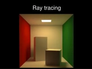
Ray Tracing • Ray tracing allows to add more realism to the rendered scene by allowing effects such as • shadows • transparency • reflections Ray Tracing
Ray Tracing • Raytracing, a simple idea: instead of forward mapping an infinite number of rays from light source to object to viewer, backmap finite number of rays from viewer through each pixel to object to light source (or other object) • Raytracing: shoot rays from eye through sample point (e.g., a pixel center) of a virtual photo • compute what color/intensity you see at the corresponding sample point on the object out there; paint this on “photo” at the ray-photo intersection point • “What you see out there” • combination of the color of the material of the surface element you hit first and the colors of light that hit it and reflect towards you Ray Tracing
Rendering with Raytracing Subproblems to solve • Generate primary (‘eye’) ray • Find closest object along ray path • find the first intersection of a ray that goes out from the eye through a pixel center (or any other sample point on image plane) into the scene • Light sample • use illumination model to determine light at closest surface element • generate ‘secondary’ rays from object Ray Tracing
Generating Rays (1/3) Ray origin • Let’s look at the geometry of the problem in untransformed world-space • We start a ray from an “eye point”: P • We send it out in some direction d from your eye toward a typical point on the film plane whose color we want to know • Points along the ray have the form P + td where • - P is the base point of the ray: the camera’s “eye point” • - d is the unit vector direction of the ray • - t is a nonnegative real number • The “eye point” is the center of projection in the perspective view volume (we use perspective coords to avoid having to deal with the inverse of a perspective transformation later) Ray Tracing
Generating Rays (2/3) Ray direction • We start raycasting with screen-space points (pixels). Need to find a point in 3-D that lies on the corresponding ray • we will use ray to intersect with the original objects in the original, untransformed world coordinate system • Transform 2D screen-space points into points on the camera’s 3D film plane • Any planes orthogonal to the look vector is a convenient film plane: constant z in canonical view volume • Choose a plane to be the film plane and then create a function that maps screen-space points onto it • what’s a convenient plane? Try the far plane :-) • to convert, we just have to scale integer screen-space coordinates into floating point values between -1 and 1 Ray Tracing
Generating Rays (3/3) Ray direction (cont.) • Transform film plane point into world-space point • - we can make the direction vector between the eye and this world-space point • - we need direction to be in world space so that we can intersect with the original object in the original, untransformed world coordinate system • Normalizing transformation takes world-space points to points in the canonical view volume • - translate to the origin, orient with the axes, scale x and y to adjust viewing angles, scale so that z: [-1, 0]; x,y: [-1, 1] • Apply the inverse of the normalizing transformation: the Viewing Transformation Ray Tracing
(A,B,C) -D (0,0,0) Ray Object Intersection (1/5) Implicit objects • If an object is defined implicitly by a function f such that f(Q) = 0 if and only if Q is a point on the surface of the object, then ray-object intersection is comparatively easy • we can define many objects implicitly • implicit functions give you potentially infinite resolution • tessellating implicit functions is more difficult than using them directly • For example, a circle of radius R is an implicit object in the plane, and its equation is • points where f(x, y) = 0 are points on the circle • An infinite plane is defined by the function: • A sphere of radius R in 3-space: Ray Tracing
Ray Object Intersection (2/5) Implicit objects(cont.) • At what points (if any) does the ray intersect the object? • Points on the ray have the form P + td • t is any nonnegative real • A point Q lying on the object has the property that f(Q) = 0 • Combining, we want to know “For which values of t is f(P + td) = 0 ?” (if any) • We are solving a system of simultaneous equations in x, y (in 2D) or x, y, z (in 3D) Ray Tracing
An Explicit Example (1/3) 2D ray-circle intersection example • Consider the eye-point P = (-3, 1), the direction vector d = (.8, -.6) and the unit circle given by: • A typical point of the ray is: • Plugging this into the equation of the circle: • Expanding, we get: • Setting this to zero, we get: Ray Tracing
An Explicit Example (2/3) 2D ray-circle intersection example (cont.) • Using the quadratic formula: • We get: • Because we have a root of multiplicity 2, our ray intersects the circle at one point (i.e., it’s tangent to the circle) • We can use the discriminant D = b2 - 4ac to quickly determine if a ray intersects a curve or not • - if D < 0, imaginary roots; no intersection • - if D = 0, double root; ray is tangent • - if D > 0, two real roots; ray intersects circle at two points • Smallest non-negative real t represents intersection nearest to eye-point Ray Tracing
An Explicit Example (3/3) 2D ray-circle intersection example (cont.) • Generalizing: our approach will be to take an arbitrary implicit surface with an equation f(Q) = 0 and a ray P + td, and plug the latter into the former: • This results, after some algebra, in an equation with t as unknown • We then solve for t, analytically or numerically Ray Tracing
Ray Object Intersection (3/5) Implicit objects-multiple conditions • For objects like cylinders, the equation • in 3-space defines an infinite cylinder of unit radius, running along the y-axis Usually, it’s more useful to work with finite objects, e.g. such a unit cylinder truncated with the limits • But how do we do the “caps?” • The cap is the inside of the cylinder at the y extrema of the cylinder Ray Tracing
Ray Object Intersection (4/5) Multiple conditions (cont.) • Picture • We want intersections satisfying the cylinder: or top cap: or bottom cap: Ray Tracing
Ray Object Intersection (5/5) Implicit surface strategy summary • Turn an implicit surface equation into an equation for t and solve • The thing you see “first” from eye point is at the smallest non-negative t-value • For complicated objects (not defined by a single equation), write out a set of equalities and inequalities and then code as cases… • Latter approach can be generalized cleverly to handle all sorts of complex combinations of objects - Constructive Solid Geometry (CSG), where objects are stored as a hierarchy of primitives and 3-D set operations (union, intersection, difference) - “blobby objects”, which are implicit surfaces defined by sums of implicit equations Ray Tracing
World-Space Intersection World space - a global view • One way to do intersection is to compute the equation of your object in world-space • Example: a sphere translated to (3, 4, 5) after it was scaled by 2 in the x-direction has equation • One can then take the ray P+td and plug it into the equation • Solve the resulting equation for t • Always start with the untransformed object definition in its own coordinate system • We then try to derive what the transformed version should be, given the CTM (call it M) • this is not easy for general transformations, and furthermore, the transformed version of the equation is always more complicated and thus more expensive to compute • can we just work with the object in its own coordinate system? Yes, as follows: Ray Tracing
MQ Q (0,0,0) Object-Space Intersection Transform ray into object-space • Express world-space point of intersection as MQ, where Q is some point in object-space: • If is the equation of the untransformed object, we just have to solve • - note d is probably not a unit vector • - the parameter t along this vector and its world space counterpart always have the same value. Normalizing d would alter this relationship. Do NOT normalize d. Ray Tracing
World-Space vs. Object-Space Use object-space if objects defined there • To compute world-space intersections, you have to transform the implicit equation of your canonical object defined in object space - often difficult • But to compute intersections in object-space, you need only apply a matrix (M-1) to P and d, which is much simpler. • does M-1 exist? • M was composed from two parts: the cumulative modeling transformation that positions the object in world-space, and the camera’s normalizing transformation • the modeling transformations are just translations, rotations, and scales (all invertible) • the normalizing transformation also consists of translations, rotations and scales (also invertible); no perspective! (Now you see why we used the “hinged” perspective view volume) • When you’re done, you get a t-value • This t can be used in two ways: • P+td is the world-space location of the intersection of the ray with the transformed object • P + td is the corresponding point on the untransformed object (in object space) Ray Tracing
Normal Vectors at Intersection Points (1/4) Normal vector to implicit surfaces • For illumination we need to find a way, given a point on the object in object-space, to determine the normal vector to the object at that point so that we can calculate angles between the normal and other vectors • If a surface bounds a solid whose interior is given by then we can find the normal vector at a point(x, y, z) via the gradient at that point: • Recall that the gradient is a vector with three components: Ray Tracing
Normal Vectors at Intersection Points (2/4) Sphere normal vector example • For the sphere, the equation is • The partial derivatives are • So the gradient is • Normalize n before using in dot products! • In some degenerate cases, the gradient may be zero, and this method fails…use nearby gradient as a cheap hack Ray Tracing
Wrong! Normal must be perpendicular Mnobject nobject Normal Vectors at Intersection Points (3/4) Transforming back to world-space • We have an object-space normal vector • We want a world-space normal vector • To transform the object to world coordinates, we just multiplied its vertices by M, the object’s CTM • Can we treat the normal vector the same way? • Answer: NO • Example: say M scales in x by .5 and y by 2 • See the normal scaling applets in AppletsLighting and Shading Ray Tracing
Normal Vectors at Intersection Points (4/4) • Why doesn’t multiplying the normal work? • For translation and rotation, which are rigid body transformations, it actually does work • Scale, however, distorts the normal in exactly the opposite sense of the scale applied to the surface, not surprising given that the normal is perpendicular • scaling y by 2 causes normal to scale by .5: • We’ll see this algebraically in the next slides Ray Tracing
Transforming Normals (1/4) Object-space to world-space • Take the polygonal case, for example • Let’s compute the relationship between the object-space normal nobj to a polygon H and the world-space normal nworld to a transformed version of H, say MH • If v is a vector in world space that lies in the polygon (e.g., one of the edge vectors), then the normal is perpendicular to the vector v: • But vworld is just a transformed version of some vector in object space, vobj. So we could write • But we’d be wrong, because v is a tangent vector • it’s transformed by the derivative… • …which includes a 3D->4D->3D mapping… Ray Tracing
Transforming Normals (2/4) Object-space to world-space(cont.) • So we want a vector nworld such that • We will show in a moment that this equation can be rewritten as • We also already have • Therefore • Left-multiplying by (Mt)-1, Ray Tracing
Transforming Normals (3/4) Object-space to world-space(cont.) • So how did we rewrite this: • As this: • Recall that if we think of vector as nx1 matrices, then switching notation, • Rewriting the formula above, we have • Writing M = Mtt, we get • Recalling that (AB)t = BtAt, we can write this: • Switching back to dot product notation: Ray Tracing
Transforming Normals (4/4) Applying inverse-transpose of M to normals • So we ended up with • Fortunately, “invert” and “transpose” can be swapped, to get our final form: • Why do we do this? It’s easier! • A hand-waving interpretation of (M3-1)t • M3 is a composition of rotations and scales, R and S (why no translates?). Therefore • so we’re applying the transformed (inverted, transposed) versions of each individual matrix in their original order • for a rotation matrix, this transformed version is equal to the original rotation, i.e., normal rotates with object • (R-1)t=R; the inverse reverses the rotation, and the transpose reverses it back • for a scale matrix, the inverse reverses the scale, while the transpose does nothing: • (S(x,y,z)-1)t = S(x,y,z)-1=S(1/x,1/y,1/z) Ray Tracing
Summary : Non-Recursive Ray Tracer P = eyePt For each sample of image Compute d for each object Intersect ray P+td with object Select object with smallest non-negative t-value(this is the visible object) For this object, find the object-space intersection point Compute the normal at that point Transform the normal to world space Use the world-space normal for lighting computations Ray Tracing
Recursive Raytracing Simulating global lighting effects (Whitted, 1979) • By recursively casting new rays into the scene, we can look for more information • Start from the point of intersection • We’d like to send rays in all directions • Send rays in directions we predict will contribute the most: • toward lights (shadow) • bounce off objects (specular reflection) • through the object (transparency) Ray Tracing
Shadows • Each light in scene makes contribution to the color and intensity of a surface element… • Iff it reaches the object! • - could be occluded by other objects in the scene • - could be occluded by another part of the same object • Construct a ray from the surface to each light • Check to see if ray intersects other objects before it gets to the light • - if ray does NOT intersect that same object or another object on its way to the light, then the full contribution of the light can be counted • - if ray does intersect an object on its way to the light, then no contribution of that light should be counted • - what about transparent objects? Ray Tracing
Iλ1 polygon 1 Iλ2 polygon 2 Transparent Surfaces (1/2) Nonrefractive transparency • For a partially transparent polygon Ray Tracing
Transparent Surfaces (2/2) Refractive transparency • We model the way light bends at interfaces with Snell’s Law Ray Tracing
Recursive Raytracing (1/2) • Trace ‘secondary’ rays at intersections: • - light: trace ray to each light source. If light source blocked by opaque object, it does not contribute to lighting, and object in shadow of blocked light at that point • - specular reflection: trace ray in mirror direction by reflecting about N • - refraction/transparency: trace ray in refraction direction by Snell’s law • - recursively spawn new light, reflection, refraction rays at each intersection until contribution negligible • Your new lighting equation… • note: intensity from recursed rays calc’d with same eqn • light sources contribute specular and diffuse lighting • Limitations • - recursive interobject reflection is strictly specular: along ray reflected about N • - diffuse interobject reflection handled by radiosity • Informative videos: silent movie on raytracing, A Long Ray’s Journey into Light Ray Tracing
Recursive Raytracing (2/2) Light-ray Trees Ray Tracing
Raytracing Pipeline • Raytracer produces visible samples from model • samples convolved with filter to form pixel image • Additional pre-processing • pre-process database to speed up per-sample calculations (done once, sometimes must be redone if objects transformed (resize, translate)) Ray Tracing
Referensi • F.S.Hill, Jr., COMPUTER GRAPHICS – Using Open GL, Second Edition, Prentice Hall, 2001 • Andries van Dam, Introduction to Computer Graphics, Slide-Presentation, Brown University, 2003, (folder : brownUni) • ______, Interactive Computer Graphic, Slide-Presentation, (folder : Lect_IC_AC_UK) Ray Tracing