Download

1 / 30
300 likes | 422 Views
Proxies of the Entire Surface Distribution of the Photospheric Magnetic Field. Xuepu Zhao http://sun.stanford.edu/~xuepu/PUBLICATION NAOC, Oct. 18, 2011. 1. Introduction.

E N D
Proxies of the Entire Surface Distribution of the Photospheric Magnetic Field Xuepu Zhao http://sun.stanford.edu/~xuepu/PUBLICATION NAOC, Oct. 18, 2011
1. Introduction • The most spectacular events with the greatest impact on the near-Earth space originate from the lower corona. To understand the various phenomena that occurred in the corona, it is crucial to determine the 3D coronal magnetic field. Unfortunately, the coronal field is notoriously difficult to measure. It has become common practice to reconstruct the coronal magnetic field from photospheric magnetic field measurement.
In all data-based coronal models and physics-based space weather prediction models, the major input is the Carrington-coordinate synoptic magnetogram map or the • Carrington magnetic synoptic map, as a proxy of the entire surface distribution of the photospheric magnetic field. • The next slice shows various types of magnetic synoptic maps. I’d like to talk about the improvement of synoptic maps made recently.
Various types of synoptic maps 1.1 Carrington Magnetic Synoptic charts (Bumba and Howard, 1965, MWO, Hoeksema, 1981, WSO) Magnetic synoptic maps (Harvey et al., 1980, KPNO) 1.2 Synoptic frame (Zhao et al., 1997; 1999; 2000, MDI, WSO) Updated synoptic maps (Arge & Pizzo, 2000, WSO) 1.3 Dynamic synoptic maps (Harvey & Wodem, 1998, KPNO Flux transportation models) Instantaneous maps (McCloughan & Durrant, 2002) Snap-shot maps (Schrijver & Derosa, 2003, MDI) Snap-shot maps (Ulrich & Boyden 2006, MWO) 1.4 Synchronic frame (Zhao et al., 2006; 2010, MDI, HMI)
2. Carrington Synoptic Maps • In constructing synoptic maps, it is implicitly assumed that the photospheric magnetic field, B(λ,φ(t),t), is stable over one solar rotation and rotating rigidly. • Magnetograms are remapped, i.e., converting magnetic field from circular disk plan into cylindrical surface in heliographic coordinate. The synoptic chart is made from central strips of remapped magnetograms observed over one solar rotation, ranging from right to left in the order of time or from left to right in the order of Carrington longitude, as show in the following figure. • Magnetic synoptic charts have been inputted into various coronal models, as inner boundary condition, and have successfully reproduced such global-scale structures as • Heliospheric current sheets and coronal holes. The updated synoptic chart has been used to predict ambient solar wind speed.
MDI WSO HMI MDI Heliographic remapped Carrington remapped WSO
Carrington rotation #2108 Magnetic Synoptic Chart (Map) A collection of 28 daily central strip Carrington longitude
3. Synoptic frame • Different from the Earth’s magnetic field, the photospheric field is not constant. In addition, many dynamic processes in the photosphere, such as flux emergence and cancellation, random-walk dispersal, meridinal advection, and differential rotation may significantly change the field distribution. Strictly speaking, the global distribution of photospheric magnetic field, B(θ,φ(t),t), is meaningful only at a specific time.
Some large-scale coronal structures, such as X ray arcades and coronal hole boundary, vary on the time scale of one day or less. To model the evolution of such coronal structures, the central synoptic frame, as a proxy of instantaneous global distribution of the photospheric field at the time of interest, may be used.
The MDI instrument on SOHO has made 2" full-disk observations of the photospheric field every 96 minutes. The high cadence MDI observations provide the possibility to monitor the change of the photospheric magnetic field that is associated with the evolution of large-scale coronal structures. By combining the MDI magnetogram observed at the time of interest and the appropriate synoptic chart, two types of the synoptic frame has been constructed: The Central synoptic frame for modeling coronal structures and the left one (Zhao et al, 1999) or Updated synoptic chart (Arge & Pizzo, 2000) for prediction of coronal and interplanetary properties.
Daily variation 96:08:23 27 96:08:24 28 96:0825 29 96:08:26 30
1994 April 14 large loop arcade over southern polar crown observed by Yohkoh SXT
Non-Force-Free Helical Field Model (Zhao et al., 2000) Free parameters: α Helical coefficient, characterizing the effect of field-aligned current a Height index , characterizing the effect of horizontal current
Based on the 1994:04:14 synoptic frame, the 1994:04:17 polar crown magnetic arcades are produced using various free parameters α and a. The magnetic arcade with α =0 & a=0.9 marches observed SXR arcade.
Using the 1994:04:17_18:27 synoptic frame and the non-force- free helical field model with a=0.9 & α=0.0, the magnetic arcade is reproduced.
4. Synchronic Frame • Synoptic frames is constructed for tracking the change of large-scale coronal structures on the time scale less than 27 days. However, there is a mapping inconsistence in synoptic frames as shown in following figure. To model coronal and heliospheric features observed simultaneously by SOHO, SDO, STEREO A and B, we improve the synoptic frame by converting synoptic-chart component observed on different time to the target time.
Black and blue vertical lines denote heliographic and Carrington longitudes. The Abscissa is in hybrid manner with heliographic longitude for magnetogram component and Carrington longitude for synoptic chart component.
The synodic rotation rate of photospheric magnetic features is latitude-dependent In deg/day It has been shown that differential rotation accounts for most of the surface transport of magnetic field over the period of one solar rotation (Worden & Harvey, 2000). Based on time difference a Carrington Longitudes from the target time we can calculate longitude shift at any latitude using Eq. (1)
5. Summary • We have shown that the magnetic elements from a synoptic map cannot be used to fill up the entire solar surface at any time within the Carrington rotation period. To fill up the whole solar surface at a specific time 41 days of observations are needed. • The central synchronic frame can be used to reproduce global coronal magnetic field and solar wind at any specific time, and monitor daily variation of large-scale coronal magnetic and plasma structures.
The left synchronic frame may be used to predict solar wind at 1 AU three days earlier than using the updated synoptic maps. • The traditional magnetic synoptic chart, though its magnetic elements cannot cover entire solar surface, can be used to reproduce gloable distribution of sector boundaries and coronal holes, implying that it is the magnetic field directly underlying the corona and heliospheric structures to be modeled that determine the above structures.