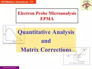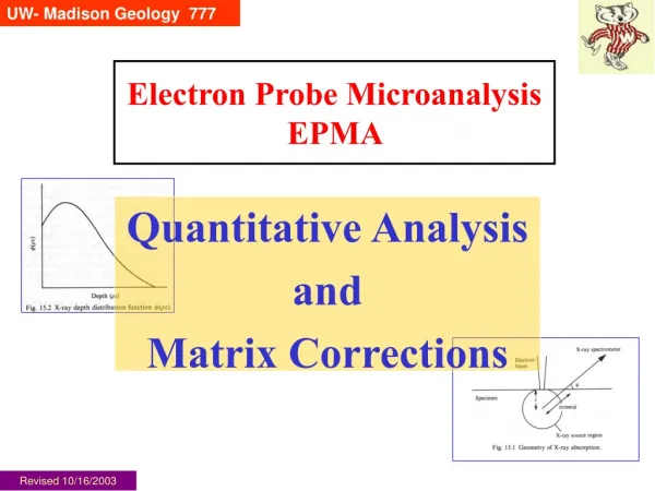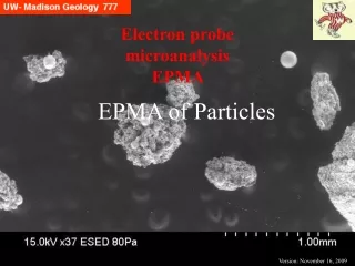
Electron probe microanalysis EPMA
Electron probe microanalysis EPMA. Processing Electron, X-ray, and CL images. Modified 8/22/08. What’s the point?. “A picture is worth a thousand words”. Raw images sometimes need to be “processed”

Electron probe microanalysis EPMA
E N D
Presentation Transcript
Electron probe microanalysisEPMA Processing Electron, X-ray, and CLimages Modified 8/22/08
What’s the point? “A picture is worth a thousand words”. Raw images sometimes need to be “processed” to highlight particular features (sometimes easy to do, sometimes difficult and requires advances computation) to extract quantitative information (e.g. modal abundances)
Image Processing & Analysis Image enhancement Segmentation and thresholding Processing in frequency space Processing binary images Image measurements Image presentation
Image Enhancement - Done Later Histogram normalization: crunching from 16 to 8 bit. This usually is a first step for visual presentation purposes, as most software packages only operate on 8 bit images. However, this does not apply for measuring absolute values of pixel intensity, such as X-ray counts. Brightness/contrast (and importantly, gamma): adjusting histogram “levels” Histogram equalization: divide intensities into equal/weighted number of categories Kernels/Rank operators: modify each pixel by some operation upon it and nearest neighbors Image math: background subtraction; ratio 2 elements Processing in frequency space (Fourier transform): removing periodic noise Applying alternate lookup tables (LUTs) for improved presentation
Intensities, Histograms, LUTs All images we are concerned with (e.g., BSE, CL, X-ray) contain one channel of information, where each constituent pixel has a value from 0 to 255 (28) or 65535 (216). These can be ordered in a histogram of intensities, with the spread defining the contrast, and the absolute values defining how bright or dark the image is. These INPUT intensities are mapped onto an OUTPUT grayscale or color table known as a Look Up Table (LUT). The transfer function is known as gamma. A gamma of 1.00 indicates a linear relationship between pixel intensities and grayscales. A gamma >1 is a non-linear function where the darker pixels are made preferentially brighter, whereas gamma <1 has the very bright pixels preferentially darkened somewhat. Adjusting only “brightness” and “contrast” controls (highlighted in many image packages) generally give poorer results compared to tweaking the gamma as part of histogram adjustment. LUT
Adjust gLevels Photoshop Brightness and Contrast: or How I Learned to Love the Histogram The original histogram is too bunched up – poor contrast. Notice the top (input) left and right sliders are not close to the min/max brightness. So we move the top (input) left and right sliders in to the min/max brightness levels.And we move the bottom (output) sliders to 10 and 254. A last (important) step is to adjust the gamma, the top middle slider. To left (higher) increases brightness of mid grays (normally the best option).
Goldstein et al, 1992, Fig. 4.53, p;. 238 The traditional imaging medium, photographic paper, has a non-linear response to light exposure through the overlying negative. Skilled darkroom technique used this to bring out subtle features in the shadows, or enhance bright features that tend to wash out. For digital images, such nonlinear processing, gamma processing, provides selective contrast Gamma Processing enhancement at either the black or white end of the gray scale, while preventing saturation or clipping of the resulting image. The signal transfer function is defined as where g is an integer (1, 2, 3, 4) or a fraction (1/2, 1/3, 1/4) and K is a linear amplification constant. For g=2, a small range of input signals at the dark end of the gray scale are distributed over a larger range of output gray levels, enhancing the contrast here; signals at the white end are compressed into fewer gray levels. For g =1/2, expansion occurs at the bright end, enhancing bright features.
One alternative/complementary procedure to manual adjust of brightness/contrast is equalization, which can be applied to the raw image. It stretches out the histogram, with the distinction that it separates the intensities into weighted bins, so that if there are a lot of pixels piled in a few bins, these bins (intensities) will have a larger number of new intensities mapped onto them – i.e., there will be “spaces” between them on the histogram, meaning those intensities will be stretched out. At the same time, bins with not many pixels in them may be squeezed together, as there is less total information relative to the high populated pixels. Histogram Levels & Equalization Russ, 1999, Fig. 4.11, p. 238.
Kernels/Rank Operators Noisy images sometimes occur for a variety of reasons, some avoidable, some not. Noise refers to some randomness added to pixel intensity values, with noise worse where count rates are low. The simplest procedure to reduce noise is to take the average of the pixel and its surrounding neighbors, and put this new average value in as the new pixel intensity. You can create a matrix with values for the coefficient by which you weigh (multiply) each pixel and adjoining neighbors. For example, one such matrix could be 1 1 1 and 1 2 1 1 1 1 another 2 4 2 1 1 1 1 2 1 These are called kernels, or rank operators. Say there was a ‘noisy’ pixel with a value of 100, when all the adjoining values were 10. The first kernel would return a new value of 20, and the ‘noise’ would be drastically reduced.
Neighborhood averaging Results of applying one kernel: a) A noisy original image, b) each 4x4 block of pixels is averaged ([less noise, but too coarse), c) each pixel replaced by average of 3x3 neighbor-hood ([ pretty nice), d) each pixel replaced by average of 11x11 neighborhood ([ less noise, but too big, causing blurring) Russ, 1999, The Image Processing Handbook (3rd edition), Fig 3.3, p. 166
The values of each pixel can be operated on (e.g. multiplied, divided, added or subtracted relative to some constant), or different elements of the same image can be operated on. The most common operations are division and subtraction. Two elements that vary together (e.g. Ca and Na in feldspar) can be divided to yield an optimized zonation map. Subtraction is useful for removing the continuum contribution, particularly for minor or trace elements. Image Math Goldstein et al, 1992, Fig 10.6, p. 535 Above is an example of false compositional contrast, an artifact of the background being a function of Z (MAN). Specimen is Al-Cu eutectic; X-ray maps are (a) Al, (b) Cu, (c) Sc. The contrast in (c) suggests Sc is present in the Cu-rich phase. However, there is no Sc, only the background in the Cu-rich phase is elevated relative to the background in the Al-rich phase. If image math is used – subtracting an additional X-ray map acquired at an off-peak (background) Sc position – a true map of Sc is seen in (d), where it is clear there is no Sc present.
Another ‘mining’ of X-ray images utilizes both the elemental information as well as the spatial (X,Y) coordinates. “Micro-Image includes a unique histogram-histogram plotting feature for unambiguous identification of numerous phases. In this screen shot, the lower right image displays a histogram-histogram plot which shows the presence of at least 6 phases including a solid solution 2 Dimensional Histograms component. The upper right image display a "traceback" of one selected phase cluster which provides black and white mask of spatial information.” (From the Advanced Microbeam Inc webpage)
Processing in Frequency Space Examples from Russ, Image ProcessingTool Kit Tutorial, Part 4, Fig 4.C.1, page 8. 4 dots and then the resulted inverted, a mask is made (center), which is then subtracted from the left FFT image. Then an inverse FFT operation is done on this image, and the result is the right image, where the noise is removed. These operations must be done on square images, using NIH Image or Russ’s Image Toolkit with Photoshop. If there periodic noise in an image (e.g., the 2 frequencies on top of the clown image), the image can be processing by a Fast Fourier Transform (FFT) of it, as is done in the small subregion in the left frame. The 2 frequencies of noise show up as 2 pairs of dots (the clown features are the NS, EW lines and center dot). If 4 small solid circles are placed upon the
Look Up Tables The mapping of intensites (e.g., BSE voltages or X-ray counts) to a displayed image uses a Look Up Table, the most common one being a gray scale. The default with MicroImage is the thermal LUT. There are many others, and you can make up your own. It is a good idea to display the LUT as a bar next to the image if they might be some confusion as to what color means what intensity. Gray scale Fire 1 Fire 2 Rainbow Ice Some LUTs from NIH Image
Processing binary images When we acquire images, we are in essence acquiring information about features – defined as compositions, or sizes or shapes, of phases or boundaries or whatever. Our eyes + brains are sorting out features constantly, such as in the process of sorting out the black lines and shapes against the white background here, translating into words and then into meanings. We can apply similar binary operations to our images – focusing on one characteristic and ignoring the rest for the moment. This is known as thresholding, where we set upper and lower thresholds of intensity (e.g., BSE) and then define as a feature (e.g., one phase) the intensities that fall in between. Software can then be applied to such a binary image to do many things, e.g., count the number of pixels (thus, determine phase area). Boolean (logical) operations can be done on sets or images, taking two element maps and create a third one that shows the regions where features containing both elements are present, or only one without the other. Morphological operations can be done to modify individual pixels within an image–apply erosion and dilation operators to separate touching phases and then count total number of separate phases or measure the dimensions or orientation of each.
Thresholding NIH Image provides an easy way to threshold images, shown here. You double click the little up/down icon (6th from top, right column) which gives you a red sliding palette that you use to color in the phase you are selecting. You then click Measure under the Analyze menu and the total number of pixels is shown in the Info Box. If you do this for all the phases Cr-spinel 57208/442225=12.9%, Mg-rich clay 215634/442225= 48.8%, Diopside 153904/442225=34.8%, Cracks 14947/442225=3.4% Total (without fudging!) = 99.9% Present, you should be able to get a total of 100±5% easily.
Making an Image into a Binary make some reasoned judgements about whether or not to include them. Here, I decided not to include them, so I then did 2 consecutive “erode” operations (under Binary menu), and then 2 consecutive “dilate” operations, to yield the final image on the right. Of course there could well be cases where you would not do the erodes. Besides being able to determine area percentages, you use the thresholded region to make a binary image of that one feature/phase. In NIH Image it is simple: Process > Binary > Make Binary. The result of that operation is shown in the center image. Note that there are some “outliers”, mainly in cracks. You need to
Binary images consist of groups of pixels selected on the basis of some common property. Logical or Boolean operations can be applied, pixel by pixel, to sets of images. The logical operations typically are AND, OR, XOR (exclusive or), NOT. The logical operator looks at each pixel to see if it is “on” or “off”. AND: requires both pixels be ON to be ON in the result. OR: if either pixel is ON, it will be ON in the result. XOR: turns a pixel ON in the result only if it is ON in only one, not both, of the images. All 3 require 2 images. The NOT operator only requires one, and it reverses the meaning of each pixel. Boolean* Operations Original X-ray maps (top): c) Si, d) Fe These have been smoothed and thresholded to make binary images. The thresholded Fe image is shown below left (a), with Fe black. The Fe and Si images have been combined as Fe AND NOT Si, to yield the right (b) image of the Fe-oxide phase, excluding the Fe-silicate phase. * From the symbolic logic developed by George Boole, British mathematician, 1815-1864 Russ, The Image Processing Handbook, 1999, Figs 7.5, 7.6, p. 436.
Si=Red, Ca=Green, K=Blue Si=Green, Fe=Red, Ti=Blue Si=Red, Fe=Green, Al=Blue Color Superposition of Elemental Maps While not strictly a Boolean operation (not binary images), by defining each elemental map with hues of either R, G or B, and then combining (flattening) the image in Photoshop, phase information can be extracted. Images from research of Josh Kearns and Jill Banfield: sand from Tanana River, central Alaska
Sometimes you want to measure features but the binary image isn’t unambiguous, as shown in the example to the right. Here, you are attempting to measure the area of the middle gray phase (a), but when you threshold it, there are outlines of the bright phase (b). The outline is only 1 pixel wide, so you can apply an erode operation, which will remove the outlines that you want to get rid of, but also it will remove the outer layer of pixels from all of the features you are interested in (c). No problem. Erosion/Dilation Just apply the dilate operation, and where there are any existing pixels, there will be added a layer of pixels (d), and now you can do your measurement. Russ, The Image Processing Handb ook, 1999, Fig. 7.36, p. 462
Geology 777 Image measurements ImageJ 1.28 NIH Image 1.63 Features in images lend themselves to measurement without too much difficulty
Software • MicroImage (interfaces with SX51) • Matrox Intellicam (interfaces with SX51 video display) • NIH/Scion Image for a manual-article-tutorial, go to rsb.info.nih.gov/nih-image/more-docs/Tutorial/Contents.html • Adobe Photoshop • Image Processing Tool Kit (Russ/Reindeer Games) – plug-ins for Photoshop • Graphic Converter (Mac) • Books • The Image Processing Handbook by John C. Russ, 3rd Ed, 1999, CRC Press (he teaches a week-long short course at North Carolina State University) • Quick Photoshop for Research, A guide to digital imaging for Photoshop 4xd, 5x,6x,7x by Jerry Sedgewick, 2002, Kluwer Academic/Plenum Publishers Resources:
Conclusion Imaging covers a wide range of topics and we have just skimmed the surface here.