Download
1 / 26
260 likes | 555 Views
Ch 6.4: Differential Equations with Discontinuous Forcing Functions . In this section focus on examples of nonhomogeneous initial value problems in which the forcing function is discontinuous. Example 1: Initial Value Problem (1 of 12). Find the solution to the initial value problem

E N D
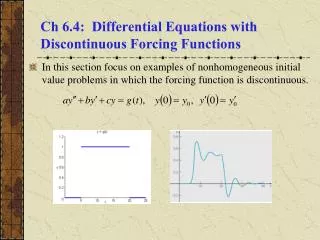
Ch 6.4: Differential Equations with Discontinuous Forcing Functions • In this section focus on examples of nonhomogeneous initial value problems in which the forcing function is discontinuous.
Example 1: Initial Value Problem (1 of 12) • Find the solution to the initial value problem • Such an initial value problem might model the response of a damped oscillator subject to g(t), or current in a circuit for a unit voltage pulse.
Example 1: Laplace Transform (2 of 12) • Assume the conditions of Corollary 6.2.2 are met. Then or • Letting Y(s) = L{y}, • Substituting in the initial conditions, we obtain • Thus
Example 1: Factoring Y(s) (3 of 12) • We have where • If we let h(t) = L-1{H(s)}, then by Theorem 6.3.1.
Example 1: Partial Fractions (4 of 12) • Thus we examine H(s), as follows. • This partial fraction expansion yields the equations • Thus
Example 1: Completing the Square (5 of 12) • Completing the square,
Example 1: Solution (6 of 12) • Thus and hence • For h(t) as given above, and recalling our previous results, the solution to the initial value problem is then
Example 1: Solution Graph (7 of 12) • Thus the solution to the initial value problem is • The graph of this solution is given below.
Example 1: Composite IVPs (8 of 12) • The solution to original IVP can be viewed as a composite of three separate solutions to three separate IVPs:
Example 1: First IVP (9 of 12) • Consider the first initial value problem • From a physical point of view, the system is initially at rest, and since there is no external forcing, it remains at rest. • Thus the solution over [0, 5) is y1 = 0, and this can be verified analytically as well. See graphs below.
Example 1: Second IVP (10 of 12) • Consider the second initial value problem • Using methods of Chapter 3, the solution has the form • Physically, the system responds with the sum of a constant (the response to the constant forcing function) and a damped oscillation, over the time interval (5, 20). See graphs below.
Example 1: Third IVP (11 of 12) • Consider the third initial value problem • Using methods of Chapter 3, the solution has the form • Physically, since there is no external forcing, the response is a damped oscillation about y = 0, for t> 20. See graphs below.
Example 1: Solution Smoothness (12 of 12) • Our solution is • It can be shown that and ' are continuous at t = 5 and t = 20, and '' has a jump of 1/2 at t = 5 and a jump of –1/2 at t = 20: • Thus jump in forcing term g(t) at these points is balanced by a corresponding jump in highest order term 2y'' in ODE.
Smoothness of Solution in General • Consider a general second order linear equation where p and q are continuous on some interval (a, b) but g is only piecewise continuous there. • If y = (t) is a solution, then and ' are continuous on (a, b) but '' has jump discontinuities at the same points as g. • Similarly for higher order equations, where the highest derivative of the solution has jump discontinuities at the same points as the forcing function, but the solution itself and its lower derivatives are continuous over (a, b).
Example 2: Initial Value Problem (1 of 12) • Find the solution to the initial value problem • The graph of forcing function g(t) is given on right, and is known as ramp loading.
Example 2: Laplace Transform (2 of 12) • Assume that this ODE has a solution y = (t) and that '(t) and ''(t) satisfy the conditions of Corollary 6.2.2. Then or • Letting Y(s) = L{y}, and substituting in initial conditions, • Thus
Example 2: Factoring Y(s) (3 of 12) • We have where • If we let h(t) = L-1{H(s)}, then by Theorem 6.3.1.
Example 2: Partial Fractions (4 of 12) • Thus we examine H(s), as follows. • This partial fraction expansion yields the equations • Thus
Example 2: Solution (5 of 12) • Thus and hence • For h(t) as given above, and recalling our previous results, the solution to the initial value problem is then
Example 2: Graph of Solution (6 of 12) • Thus the solution to the initial value problem is • The graph of this solution is given below.
Example 2: Composite IVPs (7 of 12) • The solution to original IVP can be viewed as a composite of three separate solutions to three separate IVPs (discuss):
Example 2: First IVP (8 of 12) • Consider the first initial value problem • From a physical point of view, the system is initially at rest, and since there is no external forcing, it remains at rest. • Thus the solution over [0, 5) is y1 = 0, and this can be verified analytically as well. See graphs below.
Example 2: Second IVP (9 of 12) • Consider the second initial value problem • Using methods of Chapter 3, the solution has the form • Thus the solution is an oscillation about the line (t – 5)/20, over the time interval (5, 10). See graphs below.
Example 2: Third IVP (10 of 12) • Consider the third initial value problem • Using methods of Chapter 3, the solution has the form • Thus the solution is an oscillation about y = 1/4, for t > 10. See graphs below.
Example 2: Amplitude (11 of 12) • Recall that the solution to the initial value problem is • To find the amplitude of the eventual steady oscillation, we locate one of the maximum or minimum points for t > 10. • Solving y' = 0, the first maximum is (10.642, 0.2979). • Thus the amplitude of the oscillation is about 0.0479.
Example 2: Solution Smoothness (12 of 12) • Our solution is • In this example, the forcing function g is continuous but g' is discontinuous at t = 5 and t = 10. • It follows that and its first two derivatives are continuous everywhere, but ''' has discontinuities at t = 5 and t = 10 that match the discontinuities of g' at t = 5 and t = 10.