Techniques for Continuous Space Location Problems
Explore different techniques for solving continuous space location problems, including the Median, Contour Line, Gravity, and Weiszfeld methods.


Techniques for Continuous Space Location Problems
E N D
Presentation Transcript
Outline • 11.3 Techniques for Discrete Space Location Problems • 11.3.1 Qualitative Analysis • 11.3.2 Quantitative Analysis • 11.3.3 Hybrid Analysis
Outline Cont... • 11.4 Techniques for Continuous Space Location Problems • 11.4.1 Median Method • 11.4.2 Contour Line Method • 11.4.3 Gravity Method • 11.4.4 Weiszfeld Method
11.4.1 Model for Rectilinear Metric Problem Consider the following notation: fi = Traffic flow between new facility and existing facility i ci = Cost of transportation between new facility and existing facility i per unit xi, yi = Coordinate points of existing facility i
Model for Rectilinear Metric Problem (Cont) Where TC is the total distribution cost The median location model is then to minimize:
Model for Rectilinear Metric Problem (Cont) Since the cifi product is known for each facility, it can be thought of as a weight wi corresponding to facility i.
Median Method: Step 1: List the existing facilities in non-decreasing order of the x coordinates. Step 2: Find the jthx coordinate in the list at which the cumulative weight equals or exceeds half the total weight for the first time, i.e.,
Median Method (Cont) Step 3: List the existing facilities in non-decreasing order of the y coordinates. Step 4: Find the kthy coordinate in the list (created in Step 3) at which the cumulative weight equals or exceeds half the total weight for the first time, i.e.,
Median Method (Cont) Step 4: Cont... The optimal location of the new facility is given by the jthx coordinate and the kthy coordinate identified in Steps 2 and 4, respectively.
Notes 1. It can be shown that any other x or y coordinate will not be that of the optimal location’s coordinates 2. The algorithm determines the x and y coordinates of the facility’s optimal location separately 3. These coordinates could coincide with the x and y coordinates of two different existing facilities or possibly one existing facility
Example 5: Two high speed copiers are to be located in the fifth floor of an office complex which houses four departments of the Social Security Administration. Coordinates of the centroid of each department as well as the average number of trips made per day between each department and the copiers’ yet-to-be-determined location are known and given in Table 9 below. Assume that travel originates and ends at the centroid of each department. Determine the optimal location, i.e., x, y coordinates, for the copiers.
Table 11.15 Centroid Coordinates and Average Number of Trips to Copiers
Table 11.15 Dept. Coordinates Average number of # xy daily trips to copiers 1 10 2 6 2 10 10 10 3 8 6 8 4 12 5 4
Solution: Using the median method, we obtain the following solution: Step 1: Dept. x coordinates in Weights Cumulative # non-decreasing order Weights 3 8 8 8 1 10 6 14 2 10 10 24 4 12 4 28
Solution: Step 2: Since the second x coordinate, namely 10, in the above list is where the cumulative weight equals half the total weight of 28/2 = 14, the optimal x coordinate is 10.
Solution: Step 3: Dept. y coordinates in Weights Cumulative # non-decreasing order Weights 1 2 6 6 4 5 4 10 3 6 8 18 2 10 10 28
Solution: Step 4: Since the third y coordinates in the above list is where the cumulative weight exceeds half the total weight of 28/2 = 14, the optimal y coordinate is 6. Thus, the optimal coordinates of the new facility are (10, 6).
Equivalent Linear Model for the Rectilinear Distance, Single-Facility Location Problem Parameters fi = Traffic flow between new facility and existing facility i ci = Unit transportation cost between new facility and existing facility i xi, yi = Coordinate points of existing facility i Decision Variables x, y = Optimal coordinates of the new facility TC = Total distribution cost
Equivalent Linear Model for the Rectilinear Distance, Single-Facility Location Problem The median location model is then to
Equivalent Linear Model for the Rectilinear Distance, Single-Facility Location Problem Since the cifi product is known for each facility, it can be thought of as a weight wi corresponding to facility i. The previous equation can now be rewritten as follows
Equivalent Linear Model for the Rectilinear Distance, Single-Facility Location Problem
Equivalent Linear Model for the Rectilinear Distance, Single-Facility Location Problem
Equivalent Linear Model for the Rectilinear Distance, Single-Facility Location Problem