Download
1 / 35
360 likes | 446 Views
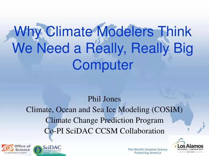
Why Climate Modelers Think We Need a Really, Really Big Computer. Phil Jones Climate, Ocean and Sea Ice Modeling (COSIM) Climate Change Prediction Program Co-PI SciDAC CCSM Collaboration. Climate System. Climate Modeling Goals.

E N D
Why Climate Modelers Think We Need a Really, Really Big Computer Phil Jones Climate, Ocean and Sea Ice Modeling (COSIM) Climate Change Prediction Program Co-PI SciDAC CCSM Collaboration
Climate Modeling Goals • Understanding processes and how they interact (only one on-going experiment) • Attribution of causes of observed climate change • Prediction • Natural variability (ENSO, PDO, NAO) • Anthropogenic climate change (alarmist fearmongering) – IPCC assessments • Rapid climate change • Input on energy policy
Climate Change IPCC TAR 2001
Greenhouse Gases • Energy production • Bovine flatulence • Presidential campaigning
State of the Art • T85 Atmosphere (150km) • Land on same • 1 degree ocean (100km) • Sea ice on same • Physical models only – no biogeochemistry • 5-20 simulated years per CPU day • Limited number of scenarios
Community Climate System Model Land LSM/CLM Atmosphere CAM NSF/DOE Physical Models (No biogeochem) 7 States 10 Fluxes 6 States 6 Fluxes 150km Once hour per per Flux Coupler hour Once 6 States 6 Fluxes 7 States 9 Fluxes 4 States 3 Fluxes 6 States 13 Fluxes day per Once per Once hour 6 Fluxes 11 States 10 Fluxes Ocean POP Ice CICE/CSIM 100km
Performance Portability • Vectorization • POP easy (forefront of retro fashion) • CAM, CICE, CLM • Blocked/chunked decomposition • Sized for vector/cache • Load balanced distribution of blocks/chunks • Hybrid MPI/OpenMP • Land elimination
Performance Limitations • Atmosphere • Dynamics (spectral or FV), comms • Physics, flops • Ocean • Baroclinic, 3d explicit, flops/comms • Barotropic, 2d implicit, comms • All • timestep
Prediction and Assessment Many century-scale simulations (>2500yrs) @~5yrs/day Cycle vampires: Many dedicated cycles at computer centers
Attribution Stott et al, Science 2000 “Simulations of the response to natural forcings alone … do not explain the warming in the second half of the century” “..model estimates that take into account both greenhouse gases and sulphate aerosols are consistent with observations over this*period” - IPCC 2001
The annual mean change of temperature (map) and the regional seasonal change (upper box: DJF; lower box: JJA) for the scenarios A2 and B2
The annual mean change of precipitation (map) and the regional seasonal change (upper box: DJF; lower box: JJA) for the scenarios A2 and B2
If elected, we plan… • High resolution • Cloud resolving atmosphere (10km) • Eddy-resolving ocean (<10km) • Regional prediction • Fully coupled biogeochemistry • Source-based scenarios • More scenarios, more ensembles • Uncertainty quantification
Resolution and Precipitation (DJF) precipitation in the California region in 5 simulations, plus observations. The 5 simulations are: CCM3 at T42 (300 km), CCM3 at T85 (150 km) , CCM3 at T170 (75 km), CCM3 at T239 (50 km), and CAM2 with FV dycore at 0.4 x 0.5 deg. CCM3 extreme precipitation events depend on model resolution. Here we are using as a measure of extreme precipitation events the 99th percentile daily precipitation amount. Increasing resolution helps the CCM3 reproduce this measure of extreme daily precipitation events.
Eddy-Resolving Ocean Obs 2 deg 0.28 deg 0.1 deg
Chemistry, Biogeochemistry • Atmospheric chemistry • Aerosols, ozone, GHG • Ocean biogeochemistry • Phytoplankton, zooplankton, bacteria, elemental cycling, trace gases, yada, yada… • Land Model • Carbon, nitrogen cycling, dynamic vegetation • Source-based scenarios • Specify emissions rather than concentrations • Sequestration strategies (land and ocean)
Atmospheric Chemistry • Gas-phase chemistry with emissions, deposition, transport and photo-chemical reactions for 89 species. • Experiments performed with 4x5 degree Fvcore – ozone concentration at 800hPa for selected stations (ppmv) • Mechanism development with IMPACT • A) Small mechanism (TS4), using the ozone field it generates for photolysis rates. • B) Small mechanism (TS4), using an ozone climatology for photolysis rates. • C) Full mechanism (TS2), using the ozone field it generates for photolysis rates. Zonal mean Ozone, Ratio A/C Zonal mean Ozone, Ratio B/C
Ocean Biogeochemistry • Iron Enrichment in the Parallel Ocean Program • Surface chlorophyll distributions in POP • for 1996 La Niña and 1997 El Niño
Global DMS Flux from the Ocean using POP The global flux of DMS from the ocean to the atmosphere is shown as an annual mean. The globally integrated flux of DMS from the ocean to the atmosphere is 23.8 Tg S yr-1 .
Increasing the deficit (1010-1012) • Resolution (103-105) • x100 horiz, x10 timestep, x5-10 vert • Completeness (102) • Biogeochem (30-100 tracers) • Fidelity (102) • Better cloud processes, dynamic land, others • Increase length/number of runs(103) • Run length (x100) • Number of scenarios/ensembles (x10)
Storage • Atmosphere • T85 29 GB/sim-yr, 0.08 GB/tracer • T170 110 GB/sim-yr, 0.3 GB/tracer • Ocean • 1 1.7 GB/sim-yr, 0.2 GB/tracer • 0.1 120 GB/sim-yr, 17 GB/tracer
Beyond Moore’s Law • Algorithms • 50% of past improvements • Tracer-friendly algorithms (inc remap advect) • Subgrid schemes • Implicit or other methods
Remapping Advection • monotone • multiple tracers free • 2nd order
Subgrid Orography Scheme • Reproduces orographic signature without increasing dynamic resolution • Realisitic precipitation, snowcover, runoff • Month of March simulated with CCSM
Comparison of sea ice shear (%/day) from CICE (a,c) and ‘old’ (b,d) models (a) (b) Feb 20, 1987 (d) (c) Feb 26, 1987
Beyond Moore’s Law • New architectures • Improved single-processor performance • Scaling vs. throughput