Typical Meteorological Year
Typical Meteorological Year. What we can learn by studying a database?. System Description. Locale. SAM. Spreadsheets. Hourly Time-Series. System Description. Locale. SAM. Spreadsheets. Hourly Time-Series. TMY3 Typical meteorological year (3 rd generation)

Typical Meteorological Year
E N D
Presentation Transcript
Typical Meteorological Year What we can learn by studying a database?
System Description Locale SAM Spreadsheets Hourly Time-Series
System Description Locale SAM Spreadsheets Hourly Time-Series
TMY3 • Typical meteorological year (3rd generation) • Data files for > 1400 U.S. sites • Each file contains 8760 hours of typical weather data • date and hour • barometric pressure • % opaque sky cover • snow depth • (more) • Also solar irradiance data • Normal direct irradiance • Diffuse horizontal irradiance • (more)
How is a TMY produced? Let’s look inside Seattle’s TMY:
How is a TMY produced? … 1970 1971 1972 1973 1974 1975 1976 1977 1978 1979 1980 1981 1982 1983 1984 1985 1986 1987 1988 1989 1990 1991 1992 1993 1994 1995 1996 1997 1998 2001 2002 2003 … Jan Feb Mar Apr May Jun Jul Aug Sep Oct Nov Dec
143Wh/m2 1397Wh/m2 683Wh/m2 extraterrestrial diffuse horizontal direct normal 546Wh/m2 In TMY3 global horizontal
Direct Normal Extinction • The atmosphere attenuates radiation by: • absorption • - lost (permanently for our purposes) • scattering • - lost direct normal, but some regained as diffuses • (We’ll explore this mathematically in a minute.)
Using these three readings to generate input to the PV • global horizontal • direct normal • diffuse horizontal q orientation of panel Input Irradiance to PV
Available Meteorological Data global horizontal direct normal diffuse horizontal Input Irradiance to PV
global horizontal direct normal diffuse horizontal HET = extraterrestrial normal at mean sun-earth distance D = D(q) = day-of-year distance correction factor Tr = transmittance due to Rayleigh Scattering Ta = tran. due to aerosol extinction Tw = tran. due to water vapor absorption To = tran. due to ozone absorption Tu = tran. due to uniformly mixed gas (O2, CO2) absorption
How do we arrive at these transmittance coefficients T λ, cfor each constituent c? • To start, let’s assume • uniform density (concentration) • we will work within a narrow wavelength window and drop the dependency onλ for now. • Each constituent, c, has an absorption coefficient, βa, and a scattering coefficient, βs, which describe the rate at which power is attenuated in a unit distance. We assume (for both of these): Beer-Bouguer-Lambert (Extinction) law – “differential form”
I0 I0 ba bs x absorption scattering
Combined Extinction Coefficient, be I0 be x extinction Beer’s law – “exponential form”
If be changes (e.g., in our “exponential atmosphere”) … I0 be = be(x) L
Transmittance and Optical Depth Tc is called the transmittance • tc is called the optical depth • unit-less, > 0 and has the path length, L, built-in • small means c transparent to light in this path • large means c blocks light in this path So we have kicked the stone down the road. If we can figure out tc we will know Tc:
( Now what? ) • We’d like to know tc for a given constituent, c. • It should be related to the volume density (ρC) of c • Experimentally, the extinction coefficient (for a given λ) is proportional to the density: kc,eis called the mass extinction coefficient of c. (ρc constant) We’re almost there: Earth’s atmosphere has an easily described air density, ρ , and our constituent’s density , ρc, should be proportional to the ρ … Beer’s law – “mass-extinction form”
The Atmospheric density is “exponential” 37% H x ρ0= air density at sea level ρ(x) = air density at x units above sea level H = 8 km, height at which density is 37% of ρ0 wc= “mixing ratio” of c in air
Now that we have density of c as a function of elevation, we can do same for extinction coefficient … … and back up one step to get optical depth: It’s an easy integral:
Correcting for angle of Sun (season/day) … θ 1 Atm sec(θ) … and recovering the transmittance: Remember – we are assuming a specific λ
We see that Tc is now expressed in terms of non-solar fields in TMY3: • x is elevation of the site • θ is an easy function of the date, lat, lon, and time • ρ0H is a function of barometric pressure • Everything else is a (constant) value in some table • This is the principle; in reality the expressions are empirically determined, but you can see the same dependences.
Example: Tu = transmittance due to uniformly mixed gas (O2, CO2) absorption. First, they define the pressure-corrected air mass Then, they compute transmittance as a function of this and the extinction coefficient: au, λ is a “tweaked” function of be(λ), which for uniformly mixed gasses is the same as ba.(λ)
We just did this: global horizontal direct normal diffuse horizontal
global horizontal direct normal diffuse horizontal Diffuse horizontal irradiance (on a clear day) will model ground albedo which makes use of snow cover. (from TMY3: snow depth and #days since last snowfall used here)
Cloud Cover • Requires different techniques since it changes quickly. • Stochastic (Monte Carlo) models need to be used. • Even good models here will not reproduce measured irradiances, even approximately. • Instead the goal is: • Monthly moments (mean, variance, skewness, kurtosis) • Monthly CDFs. • Preservation of correlations and cross-correlations between the above three modeled values. • All non-deterministic algorithms
That’s it, but -- -- I wrote a short visualization demo. What’s in the file on Jan 14? Let’s look at this data in 3D …