Download
1 / 36
390 likes | 559 Views
Ch 5. Initial Display Alternatives and Scientific Visualization. AM www.Remote-Sensing.info. Initial Display Alternatives and Scientific Visualization. Scientists interested in displaying and analyzing remotely sensed data actively participate in scientific visualization , defined as:

E N D
Ch 5. Initial Display Alternatives and Scientific Visualization AM www.Remote-Sensing.info www.Remote-Sensing.info
Initial Display Alternatives and Scientific Visualization Scientists interested in displaying and analyzing remotely sensed data actively participate in scientific visualization, defined as: “visually exploring data and information in such a way as to gain understanding and insight into the data”. The difference between scientific visualization and presentation graphics is that the latter are primarily concerned with the communication of information and results that are already understood. During scientific visualization we are seeking to understand the data and gain insight.
Initial Display Alternatives and Scientific Visualization • Scientific visualization of remotely sensed data is still in its infancy. Its origin can be traced to the simple plotting of points and lines and contour mapping. • We have the ability to conceptualize and visualize remotely sensed images in 2D space in true color (2D to 2D). • We can drape remotely sensed data over a digital terrain model (DEM) and display the synthetic 3D model on a 2D map or computer screen (i.e., 3D-2D). • If we turned this same 3D model into a physical model that we could touch, it would occupy the 3D to 3D portion of scientific visualization mapping space. • This discussion identifies the challenges and limitations associated with displaying remotely sensed data and makes suggestions about how to display and visualize the data using black-and-white and color output devices.
Temporary Video Image Display • Bitmapped Graphics • The digital image processing industry refers to all raster images that have a pixel brightness value at each row and column in a matrix as being bitmapped images. The tone or color of the pixel in the image is a function of the value of the bits or bytes associated with the pixel and the manipulation that takes place in a color look-up table. • For example, the simplest bitmapped image is a binary image consisting of just ones (1) and zeros (0).
Jensen, 2004 • The brightness value of a picture element (pixel) is read from mass storage by the central processing unit (CPU). The digital value of the stored pixel is in its proper i,j location in the image processor’s random access memory (RAM), often referred to as a video frame buffer. The brightness value is then passed through a black-and-white or color look-up table where modifications can be made. The output from the digital color look-up table is passed to a digital-to-analog converter (DAC). The output from the DAC determines the intensity of the signal for the three guns (Red, Green, and Blue) in the back of the monitor that stimulate the phosphors on a computer cathode-ray tube (CRT) at a specific x,y location or the transistors in a liquid crystal display (LCD).
RGBColor Coordinate System Digital remote sensor data are usually displayed using a Red-Green-Blue (RGB) color coordinate system based on additive color theory and the three primary colors of red, green, and blue. Additive color theory is based on what happens when light is mixed, rather than when pigments are mixed using subtractive color theory. For example, in additive color theory a pixel having RGB values of 255, 255, 255 produces a bright white pixel. Conversely, we would get a dark pigment if we mixed equally high proportions of blue, green, and red paint (subtractive color theory). Using three 8-bit images and additive color theory, we can display 224 = 16,777,216 color combinations. RGB brightness values of 255, 255, 0 would yield a bright yellow pixel, and RGB brightness values of 255, 0, 0 would produce a bright red pixel. RGB values of 0, 0, 0 yield a black pixel. Grays are produced along the gray line in the RGB color coordinate system when equal proportions of blue, green, and red are encountered (e.g., an RGB of 127, 127, 127 produces a medium-gray pixel on the screen or hard-copy device). Jensen, 2004
Color Look-up Tables: 8-bit How do we control the exact gray tone or color of the pixel on the computer screen after we have extracted a byte of remotely sensed data from the mass storage device? The gray tone or color of an individual pixel on a computer screen is controlled by the size and characteristics of a separate block of computer memory called a colorlook-up table, which contains the exact disposition of each combination of red, green, and blue values associated with each 8-bit pixel. Evaluating the nature of an 8-bit image processor and associated color look-up table provides insight into the way the remote sensing brightness values and color look-up table interact. Jensen, 2004
Color Density Slice of the Thematic Mapper Band 4 Charleston, SC Image
Color Density Slice of the Thermal Infrared Image of the Savannah River
Class Intervals and Color Lookup Table Values for Color Density Slicing the Pre-dawn Thermal Infrared Image of the Savannah River
Color Density Slice of the Thermal Infrared Image of the Savannah River
Optimum Index Factor Ranks the 20 three-band combinations that can be made from six bands of Landsat TM data (not including the thermal-infrared band). Band combination: 1,2,3 1,2,4 1,2,5 1,2,6 2,3,4 2,3,5 2,3,6 3,4,5 3,4,6 etc. Where sk is the standard deviation for band k, and rjis the absolute value of the correlation coefficient between any two of the three bands being evaluated. The largest OIF will generally have the most information (as measured by variance) with the least amount of duplication (as measured by correlation). Applicable to any multispectral dataset.
Optimum Index Factor Ranks the 20 three-band combinations that can be made from six bands of Landsat TM data Band combination: 1,2,3 Band combination: 3,4,5 Better
Sheffield Index A statistical band selection index based on the size of the hyperspace spanned by the three bands under investigation. Sheffield suggests that the bands with the largest hypervolumes be selected. The index is based on computing the determinant of each p by p sub-matrix generated from the original 6 6 covariance matrix (if six bands are under investigation). The Sheffield Index (SI) is: where is the determinant of the covariance matrix of subset size p. In this case, p = 3 because we are trying to discover the optimum three-band combination for image display purposes. The SI is first computed from a 3 3 covariance matrix derived from just band 1, 2, and 3 data. It is then computed from a covariance matrix derived from just band 1, 2, and 4 data, etc. This process continues for all 20 possible band combinations if six bands are under investigation, as in the previous example. The band combination that results in the largest determinant is selected for image display. All of the information necessary to compute the SI is actually present in the original 6 6 covariance matrix. The Sheffield Index can be extended to datasets containing n bands. Band combination: 1,2,3 1,2,4 1,2,5 1,2,6 2,3,4 2,3,5 2,3,6 3,4,5 3,4,6 etc.
Merging Remotely Sensed Data • Band Substitution • Color Space Transformation and Substitution • RGB to IHS Transformation and back again • Chromaticity Color Coordinates System • and the Brovey Transformation • Principal Component Substitution • Pixel-by-pixel Addition of High-Frequency • Information • Smoothing Filter-based Intensity Modulation • Image Fusion Jensen, 2004
Merging Different Types of Remotely Sensed Data for Effective Visual Display • All data sets to be merged must be accurately registered to one another and resampled to the same pixel size. Several alternatives exist for merging the data sets, including: • Simple band substitution methods • Color space transformation and substitution methods using various color coordinate systems. • Substitution of the high spatial resolution data for principal component #1.
Merging Remotely Sensed Data Using the Band Substitution Method
Color Composite of Marco Island, Florida SPOT Imagery October 11, 1988 Created using the band substitution method: R = SPOT band 3 (NIR) 20 m G = SPOT band 4 (Pan) 10 m B = SPOT band 1 (Green) 20 m
Merging Remotely Sensed Data • Color Space Transformation and Substitution • RGB to IHS Transformation and back again • Chromaticity Color Coordinates System • and the Brovey Transformation • Principal Component Substitution • Pixel-by-pixel Addition of High-Frequency • Information • Smoothing Filter-based Intensity Modulation • Image Fusion Jensen, 2004
Merging Different Types of Remotely Sensed Data for Effective Visual Display Intensity-Hue-Saturation (IHS) Substitution: IHS values can be derived from the RGB values through the transformation equations: Substitute Intensity data from the IHS transformation for one of the bands, e.g., RGB = 4, I, 2
Chromaticity Color Coordinate System • A chromaticity color coordinate systemcan be used to specify color.The coordinates in the chromaticity diagram represent the relative fractions of each of the primary colors (red, green, and blue) present in a given color. Since the sum of all three primaries must add to 1, we have the relationship: • or • Entry into the chromaticity diagram is made using the following relationships: • where R, G, and B represent the amounts of red, green, and blue needed to form any particular color, and x, y, and z represent the corresponding normalized color components, also known as trichromatic coefficients. Only x and y are required to specify the chromaticity coordinates of a color in the diagram since x + y + z = 1. Jensen, 2004
Chromaticity Diagram
Image Merging using the Brovey Transform • The Brovey transform may be used to merge (fuse) images with different spatial and spectral characteristics. It is based on the chromaticity transform and is a much simpler technique than the RGB-to-IHS transformation. The Brovey transform also can be applied to individual bands if desired. It is based on the following intensity modulation: • where R, G, and B are the spectral band images of interest (e.g., 30 30 m Landsat ETM+ bands 4, 3, and 2) to be placed in the red, green, and blue image processor memory planes, respectively, P is a co-registered band of higher spatial resolution data (e.g., 11 m IKONOS panchromatic data), and I = intensity. Jensen, 2004
Image Merging using Band Substitution, Principal Components Substition, and the Brovey Transform
Image Merging using Principal Component Substitution • Chavez et al. (1991) used principal components analysis applied to six Landsat TM bands. The SPOT panchromatic data were contrast stretched to have approximately the same variance and average as the first principal component image. The stretched panchromatic data were substituted for the first principal component image and the data were transformed back into RGB space. • The stretched panchromatic image may be substituted for the first principal component image because the first principal component image normally contains all the information that is common to all the bands input to PCA, while spectral information unique to any of the input bands is mapped to the other n principal components.