Download

1 / 17
190 likes | 333 Views
This paper discusses the challenge of calculating the 0.5th percentile of an insurer's net assets, a critical task for determining Value at Risk (VaR). Utilizing Radial Basis Functions (RBF) for approximation, the authors demonstrate how RBFs can outperform traditional polynomial methods, especially in high-dimensional spaces. The study covers simulation techniques, the necessity for robust approximation in insurance modeling, and the implications of using different basis functions depending on data characteristics. Results show RBF performs better in terms of accuracy and adaptability compared to polynomials.

E N D
Approximation of heavy models using Radial Basis Functions Graeme Alexander (Deloitte) Jeremy Levesley (Leicester)
The problem • Calculate Value at Risk • Need to determine 0.5thpercentile of insurer’s net assets in one year • Net assets = f(R1,R2,R3,...Rn) • Many firms have previously calculated the percentiles of univariatedistns, and aggregated using correlation matrix / copula approach
Moving to Solvency II • For internal model approach, strongly encouraged to calculate the whole distribution of Net Assets, not just the percentile • It is a simple matter to generate 100,000 simulations of (R1,R2,..Rn) • However, evaluating f(r1,r2,..rn) for a single realisation of the risk vector using the “heavy model” can take hours!! • Common approach: Run the heavy models on a small number of points, and interpolate to obtain estimator function fE(r1, r2, ..,rn), known as a “lite model”
Splines Linear spline approximation to sin(x) Combination of hat functions
Cubic Splines Cubic spline approximation to sin(x) Combination of B-splines
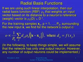
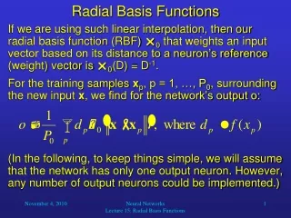
Radial basis function approximation • Set of points • A basis function • Approximation
More generally Data Y x Gaussian y
How to compute coefficients Interpolation Linear Equations
An Example - annuity • Difficult to test our interpolation on real-life data due to the length of time it takes to run heavy models • So let’s take a simple product, a single life annuity, £1 payable p.a. • Assume just two risk factors, discount rate and mortality • Assume a constant rate of mortality 1/T in each future year. Thus, the cash flows are: (T-1)/T at the end of year 1, (T-2)/T at end of year 2,1 / T at end of year T-1 • Allow T and disc to vary stochastically • disc~ N (8%, 2.5%2) • T ~ N (20,9)
An Example - annuity • We used 10 fitting points. • It turns out that the polynomial function (order 3) performs slightly better than the RBF 99.5th percentile of liability: Actual = 9.27 RBF (Gaussian) estimate = 8.86, error = 4% Polynomial estimate = 9.25, error = 0.19%
What if there is a discontinuity? Chart shows liabilities against T, for fixed disc=8%: Was fitted using “norm” function. Unlikely to arise in practice, though. However....
Choice of polynomial or RBF • Choice of appropriate polynomial terms is problematic. High degree polynomials are famously unstable (Gibb’s phenomena) • Choice of RBF is related to the “smoothness of the data” – see difference between Gaussian and norm function. This requires some user input, but does not require other experimentation. • RBF is adaptable to the placement of new points near to where error is being observed in approximation. This is not robust with polynomial approximation.
With profits • The realistic balance sheet includes a “cost of guarantees” • For example, suppose there is a guaranteed sum assured on the assets, equal to £500. • Crudely, we can model the cost of guarantees as a put option on the asset share. • Assume that: • Asset Share is £1,000 • Strike price (guarantee) is £500 • Assets ~ N (1000, 3002), disc~ N (8%, 2.5%2) This time the radial basis function (“norm”) does better: Actual = £83.53 RBF estimate = £74.6, error = 11% Polynomial estimate = £1,735, error = 1978%
With profits • Polynomial has difficulty coping with the particular behaviour shown • Also, the fitting problem is prone to becoming singular • RBF (using “norm”) does much better
Smoothing splines • If the data is noisy • Minimise • Choice of l is crucial
Summary • It is worthwhile to explore the use of radial basis functions for approximation. • They are good in high dimensions, and adapt easily to the local shape of the surface. • Polynomials are good where the surface is close to a polynomial in reality • They are also difficult to implement in high dimensions. • There are different RBFs and different approximation processes depending on the nature and reliability of the data.