Modified Rational Method for Texas Watersheds
Modified Rational Method for Texas Watersheds. Runoff coefficients from Land use. 90 watersheds in Texas for us to estimate standard (table) rational runoff coefficient using ArcGIS

Modified Rational Method for Texas Watersheds
E N D
Presentation Transcript
Runoff coefficients from Land use • 90 watersheds in Texas for us to estimate standard (table) rational runoff coefficient using ArcGIS • From a previous TxDOT project, we had a geospatial database containing watershed boundaries for 90 Texas watersheds, which were delineated using 30-meter Digital Elevation Model (DEM). • National Land Cover Data (NLCD) for 2001 were obtained for the Texas from the USGS website http://seamless.usgs.gov/. • The first task was to cut out the NLCD layer using watershed boundary for a particular watershed and find out areas of different classes of land cover within that watershed. • Clipping polygon method was used using original NAD_1983_Albers projected coordinate system.
Runoff coefficient contd.. • For clipping polygon method Raster NLCD layer converted into the polygon feature layer. • The “Clip” function of the Arc Toolbox used by selecting “Analysis Tools”, then “Extract”. • “Input Features” should be 2001 NLCD panel containing selected watershed, “Clip Features” should be the layer containing selected watershed boundary, and “Output Feature Class” is to provide a shape file name for storing clipped NLCD area. • The attribute table was opened, “Area” field added and then Calculate Geometry function was used to determine the areas for different grid (land cover) codes. • Using the Statistics and Summarize functions, the total area as well as the individual area of each land cover class for the watershed was obtained.
Runoff coefficient contd.. • Each different watershed has different land cover classes distributed inside its watershed boundary. • It was found that there were total 15 land cover classes involved for the 90 watersheds studied. • Our next task was to assign runoff coefficient for particular land cover class. • From different literature sources studied, typically we do not find runoff coefficients for most of 15 NLCD land-cover classes, but we identified similar land use types to match them. • Assuming that all of the rainfall is converted into runoff for open water and wetlands, the value of C assigned to these land-cover classes is 1. • For the other land cover classes a range of C values are available in the mentioned sources under similar land use types. • Average values were assigned for them after determining under which land use type the particular class falls or closely matches.
Runoff coefficient contd.. • A weighted C value was calculated in excel spreadsheet for each watershed using the following equation: • Weighted C value compared with “Table C” values and observed runoff coefficient values from Kirt Harle (2003) and from another TxDOT project supervised by Dr. David B. Thompson for 36 watersheds.
Future work for runoff coefficient • Our rainfall and runoff data were in the range of date from 1960-1980. • True Land cover conditions of that time will be represented by the older NLCD. • Reliable NLCD as old as 1992 is found. • Repetition of the work for runoff coefficient calculation using the NLCD 1992 has started.
Modified Rational Method • For MRM three different possible types of hydrograph can be developed for the given sub-basin. When rainfall duration = tc(from Wanielista, Kersten and Eaglin)
When rainfall duration > tc Assumptions of rainfall distribution and rainfall loss: (1). Uniform rainfall distribution (2). No initial loss (3). Constant rainfall loss over the duration
(“Urban Surface Water Management” by Walesh, 1989) • When rainfall duration < tc • MRM can be extended to applications for nonuniform rainfall distribution. • The runoff hydrograph from the MRM for the rainfall event with the duration less than the time concentration can be converted to a unit hydrograph (UH). • UH generated can be used to obtain runoff hydrographs for any nonuniform rainfall events using unit hydrograph theory (convolution).
Rational Hydrograph Method (RHM) proposed by Guo (2000, 2001) for continuous nonuniform rainfall events. • RHM was used to extract runoff coefficient and time of concentration from observed rainfall and runoff data through optimization. • Considered the time of concentration as the system memory (Singh 1982) and used a moving average window from (T-tc) and T to estimate uniform rainfall intensity for the application of the rational method to determine hydrograph ordinates. • For 0 ≤ T < tc • For tc ≤ T ≤ Td (the rainfall duration) • For Td ≤ T ≤ (Td+Tc), Guo (2001) adopted linear approximation for a small catchment
A hypothetical non-uniform rainfall event tested with 5-min MRM unit hydrograph and then with Guo’s RHM . • DRH predicted by the two methods show some differences after the rainfall ceases. • Guo’s RHM (2002, 2001) used a linear approximation from the discharge Q(Td) at the end of the rainfall event to zero at the time Td + Tc. • For nonuniform rainfall events this approximation is not correct because this will result the violation of the conservation of volume for the rainfall excess and the runoff hydrograph.
Huo et al. (2003) extended the rational formula to develop design hydrographs for small basins for nonuniform rainfall inputs using the following design rainfall intensity formula: • Used an extended rational formula proposed by Chen and Zhang (1983) to compute the design peak flow (Qm,p) with design frequency of p and time of concentration (tc): • V. P. Singh and J. F. Cruise (1982) used a systems approach for the analysis of rational formula. • Watershed represented as a linear, time-invariant system . • Nash (1958) equation used to obtain instantaneous unit hydrograph (IUH). • for 0 ≤t ≤Tc . • for t≥ Tc • Used the convolution to derive the D-hr unit hydrograph.
A symmetric trapezoidal shape unit hydrograph obtained for D<Tc . • for 0 ≤t ≤D • for D ≤t ≤Tc • for Tc ≤t ≤Tc + D • Concluded probability density function (PDF) of the rational method is a uniform distribution with entropy increasing with the increasing value of Tc.
MRM UH development and convolution • For all the 90 watersheds the unit hydrograph duration (d) used is 5 minutes. • Time of concentration obtained from the square root of area of the watersheds. • We also have Tc developed using Kirpich method from three other sources: LU, UH and USGS. • We have runoff coefficients obtained from two methods Cvlit and Cvbc. • Fortran code is developed to calculate the rainfall excess and finally perform convolution to get DRH. • Different combinations of runoff coefficient and time of concentration used to get different simulated results of DRH.
Seventeen error parameters between observed and predicted DRHs were calculated after applying MRM UH to each event. • Average/SD error parameters were estimated for all events in the same station. • Some of the events were selected randomly to plot the observed and modeled DRH. • Plot was made between the peak value of the modeled and observed discharges. • Plot was made between the relative time to peak between the modeled and observed data.
Statistical error parameters Nash - Sutcliffe efficiency (ME) and the coefficient of determination (R2) were calculated for each run. • Gamma UH was also developed using the regression equations with MRNG Optimized Qp and Tp (Pradhan 2007) of UH. • Mean Gamma UH developed were applied to all the events corresponding to the same station to generate DRHs by convolution. • Two runs were made one with Cvbc and then with Cvlit .
Statistical summary of peak discharge results using Cvbc and different Tc
Statistical summary of time to peak results using Cvbc and different Tc
Statistical summary of peak discharge results using Cvlit and different Tc
Statistical summary of time to peak results using Cvlit and different Tc
Statisticalsummary of peak discharge results using Gamma UH and different C
Statistical summary of time to peak results using Gamma UH and different C