Download
1 / 15
150 likes | 337 Views
A Computational Study of Stochastic Models in Finance. Christopher MacLellan Undergraduate Research Day April 26, 2008. To computationally simulate Brownian motion and Geometric Brownian motion To understand the assumptions that need to be made for the Black-Scholes model

E N D
A Computational Study of Stochastic Models in Finance Christopher MacLellan Undergraduate Research Day April 26, 2008
To computationally simulate Brownian motion and Geometric Brownian motion To understand the assumptions that need to be made for the Black-Scholes model To Computationally simulate the Black-Scholes / Black-Scholes-Merton call and put options Research Objectives
Brownian motion: continuous-time stochastic process first recognized by Robert Brown, a British botanist. First observed in grains of pollen suspended in water Later represented Mathematically by Norbert Wiener as: W j= W j−1dW j , j=1,2,... , N where dWj is an independent random variable of the form ( t) N 0,1 Brownian Motion
Geometric Brownian motion: A stochastic process that follows a geometric (exponential) Brownian motion. Represented by the equation dSt = St dt St dWt where Wt is a Brownian motion and (percentage drift) and (percentage volatility) are constants. Geometric Brownian motion
Single Brownian motion Multiple Brownian Motion Brownian Motion Simulated
Geometric Brownian Motion Geometric Brownian Motion Simulated
Call Option- Gives the holder the right to buy an asset at a later time for a predetermined price. Example: If I have an option for the right to buy a share of a stock that is currently valued at $100/share for $105/share a week from now and that stock jumps to $110/share I can exercise the option and buy the shares at $105/share instead of $110/share thus saving myself $5 European Call Options
Put Option- Gives the holder the right to sell an asset at a later time for a predetermined price Example: If I have an option for the right to sell a share of a stock that is currently valued at $100/share for $95/share a week from now and that stock drops to $90/share I can exercise the option and sell the shares at $95/share instead of $90/share thus saving myself $5. European Put Option
The price of an option is essentially the dollar value for the risk associated with the option. As someone selling an asset if you price the risk too low then you will lose money. If you price it too high no one will buy the option. Price of the Option
Black-Scholes is used to establish a riskless portfolio. This can be done because the stock price and the option price are both directed by the same force: stock price movements. In the short term a call option is perfectly positively correlated with the price of the underlying stock. In the short term a put option is perfectly negatively correlated with the price of the underlying stock Black-Scholes
the price of the asset follows a geometric Brownian motion it is possible to sell the underlying asset short. there is no arbitrage trading is continuous there are no transaction costs or taxes all securities are divisible (you can buy fractions of shares) you can always borrow and lend cash at a constant risk free interest rate the stock does not pay dividends Black-Scholes Assumptions
Call Option C S , T =S d1−K e−r T d2 Put Option P S , T =K e−r T −d2 −S −d1 Supporting Equations from Black Scholes Formula d1=ln S / K r 2 /2 T / (T) d2 =ln S / K r − 2 /2 T / (T) Option Prices using Black Scholes
Brownian motion is important for modeling random movement in nature including the stock market Geometric Brownian motion is what one would use in Stock Market modeling because it follows an exponential growth curve. Options Priced with the Black Scholes model make money or break even but only under certain assumptions Conclusion
Modifying the model to include transaction costs Modifying the model to include stocks that pay dividends (American Options) Determining if there are anyways to even more closely value the price of an option considering this model assumes a LogNormal Distribution (Geometric Brownian Motion) Future Research