Download
1 / 20
210 likes | 353 Views
Statistical Parametric Mapping. Lecture 10 - Chapter 12 Preparing fMRI data for statistical analysis. Textbook : Functional MRI an introduction to methods , Peter Jezzard, Paul Matthews, and Stephen Smith. Many thanks to those that share their MRI slides online.

E N D
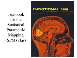
Statistical Parametric Mapping Lecture 10 - Chapter 12 Preparing fMRI data for statistical analysis Textbook: Functional MRI an introduction to methods, Peter Jezzard, Paul Matthews, and Stephen Smith Many thanks to those that share their MRI slides online
Figure 12.1. Average fMRI from finger study and its k-space magnitude representation (both for the same slice). k-space values are log10 of raw values Reconstruction of slice-by-slice real and imaginary k-space images was done on the MRI system (Siemens 3T Trio). Raw data can be accessed for k-space processing if needed.
k-space processing • Ghost correction • additional readouts without phase encoding to calculate shifts in readout directions • phase/amplitude compensation for physiological noise • translation for some registration by applying first order phase shift
Slice Timing • No within slice correction (<100 msec). Slices corrected to time of first slice in the volume. All slices in corrected image volume appear to have been collected simultaneously. • Correction often done using phase shift applied following FFT then transforming back to time domain using FFT-1. Provides more accurate interpolation. • Assumes slices remain spatially aligned throughout time course • motion must be corrected (another chapter) • motion induced distortions must be corrected where F(f) is the Fourier transform of f(t), the time course signal. The phase correction term is straightforward to calculate since the time to shift (dt) is known from pulse sequence information.
Spatial Filtering • Used to improve SNR • signal ranges from 0.5-5% so to achieve SNR of 10:1 need noise to range from 0.05-0.5% of the mean signal. • Spatial filtering increases spatial correlation by averaging within a neighborhood of each data point (kernel extent) • Can be implemented in Fourier domain (as multiplication) or spatial domain (as convolution), but spatial domain is simple for small extent filters. • Spatial domain filtering is usually separable such that 2D filtering can be done using a 1D filter along x followed by a 1D filter along y. • Similarly 3D filtering can be done by three orthogonal passes over the data by a 1D filter. • 3D convolution uses 27 multiplications and addadditiona for each point for a 3x3x3 kernel, while three sequential 1x3 filters use only 9. • ratio = nD-1/D (n2/2 for 3D) where D is the number of dimensions and n is the filter extent in one dimension. • For large n Fourier filtering is more efficient. • Filtering in the slice direction often not needed with fMRI because large slice thickness provides this. • If filtering is done in slice direction use caution since many filter kernels are not specified in mm but rather by index.
Figure 12.2. Three examples of Gaussian filter profiles. Wider filters provide more smoothing and have a lower peak value, since they are normalized to be unit area. where = FWHM/2.35 and x is distance from the central peak.
FWHM Figure 12.4. Gaussian filters can be implemented using either frequency or spatial domain versions. Spatial domain filtering is done using finite widths (kernel extent) fitted to a Gaussian function. Here data spacing is 3 mm but the FWHM of the filter is 10 mm. This filter is truncated to a kernel size of 7 and the outer points reduced for a smoother response. Smoothing filters must be unit area (sum of weights = 1). Frequency domain versions will have kernel size = image dimension.
Figure 12.3. fMRI slice before and after 2D filter with Gaussian filter with FWHM = 4 mm. Kernel was 7x7 pixels. 2D filter used slice thickness was 5 mm. High pixel values tend to be reduced and low pixel values increased by the spatial averaging.
FWHM = 40 mm 20 mm 10 mm 5 mm 0 mm Figure 12.5. Significant clusters of activations (Z>2.3, P<0.01). Red is visual and blue is auditory stimulation. Small clusters are either lost or merged into larger clusters with increasing filter size.
Value Normalization • Very important for PET O-15 CBF studies where differences in activity, decay, etc. must be removed before processing. • fMRI Methods • adjust each volume image (timepoint in time series of volumes) to same mean brain value (threshold or shrinkwrap ROI to brain first) • adjust to same median value • adjust to same WM value (i.e. not activation dependent) • do not perform value normalization • include volume mean values as covariate in GLM • Problems • the BOLD signal increases activations so image volume average value rises and scaling to compensate reduces all pixel values • attenuates activations • non-activated voxels can appear as reductions instead of non-significant change. • processing without value normalization is appropriate for this case • with studies that induce whole-brain shifts in blood flow such as blocks with varying levels of CO2 value normalization would tend to remove the global shift • processing without value normalization is appropriate for such studies • In multi-subject studies adjust 4D data from each subject to have the same value
Figure 12.6. Whole brain histograms of z-scores in statistical parametric images for four different value normalization methods. Only result using no value normalization show a correctly aligned zero centered plot. Due to asymmetry induced with positive activations the other methods tend to shift the histograms to the left.
L R fMRI average image (left) and z-score statistical parametric image following statistical analysis. Note the large region of increased signal in the hand motor area (task was right finger movement).
Finger movement z-statistic image. Max: z = 11.24 Min: z = -6.77 Histogram of the z-stat image. Red line shows z = 0. Value normalization shows distribution shifted to the left of zero (red line).
Temporal Filtering • Temporal filtering is applied to voxel time course data • The goal is to preserve signal frequencies of interest (those elicited by design) while removing low and high frequency noise (not elicited by design) • Low frequency noise shifts baseline and can be due to machine drift. Remove to optimally fit the signal components of interest in the study • High frequency noise impacts temporal SNR especially for short duration activations and short design blocks • Periodic physiological signals (cardiac) might be aliased into the frequency range of interest • aliasing occurs when sampling rate fs (1/TR) is less than 2X the frequency of the unwanted signal (fu) • aliased frequency fa = fs – fu • if fs = 1 Hz (TR=1 s) and heart frequency fu = 1.1 Hz then fa = -0.1 Hz • This corresponds to a periodic signal with period = 10 sec which might be close to that of the tasks so standard filtering would reduce the task signal. • Fully satisfactory solutions not yet available, so best to avoid by careful selection task periods. May not have as much control of TR.
Figure 12.7. Decomposition of raw time course into signal of interest and low and high frequency noise. Signal of interest is that resulting from task design pattern. Failure to account for low frequency leads to higher residual errors in GLM. Removal of high frequncy noise can improve fit.
Temporal Filtering Figure 11.8. Time course of single voxel before temporal filtering (top) and after filtering and overlaying of the expected time course model. High-pass filtering removes low frequency non-physiologic modulation of activations in this example. Baseline was restored in this example.
High-Pass Temporal Filtering • Remove Low frequency noise • Preserve frequency range of interest • filter cutoff frequency (fc) should be lower than frequency range of interest • filter cutoff period (1/fc) should be longer than that of stimulation blocks (1.5X suggested) • mixed blocks ABACABAC (A is rest) each of 10 time points: • when comparing AB or AC cutoff period ~1.5x 2x 10 • when comparing AB to AC cutoff period ~ 1.5x 4x 10
High-Pass Temporal Filtering • High-Pass (HP) filter can be synthesized as HP(f) = 1 - LP(f) • In temporal domain this is implemented as S(t) - G(t)S(t) where is the symbol for convolution and G(t) is a Gaussian LP filter. Simply stated the high-pass filtered time series can be calculated by subtracting the low-pass filtered time series from the unfiltered time series. In some fields this filtering strategy is called unsharp masking. • Linear filters can induce negative temporal correlations • Non-linear HP filter • running linear fit over filter extent (period) • ignores shorter period fluctuations • deals well with some forms of outliers • output is value predicted at central time point from fitted line • Gaussian weighting can be used to deemphasize points away from the central time point
Low frequency High frequency Figure 12.8. Magnitude response of three high-pass temporal filters. Graph runs from short periods (high frequencies) to long periods (low frequencies). The response is near unity for periods < 10 for all three filters (range of interest here). The Butterworth filter drops off more rapidly (half response at period ~ 12 while the others drop off more gradually with half response at period ~ 22).
APPENDIX Figure 12.9. Graphical demonstration of convolution of Gaussian spread function with a square wave input signal. Gaussian spread function’s center is offset from the origin (t=0) to simulate delay in response. Note origin is shifted to right side by the reflection done during convolution. Output signal is indexed by location of this shifted origin. In this example the value of the output signal is the average within the overlapping (black) region since signal is zero outside that range.