Main idea: to tackle the complexity of biological systems investigate Programming Theory Concepts

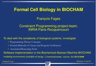
1. Formal Verification and Inference of Biochemical Models François FagesConstraint Programming project-team, INRIA Paris-Rocquencourt, France • Main idea: to tackle the complexity of biological systems investigate • Programming Theory Concepts • Formal Methods of Circuit and Program Verification • Automated Reasoning Tools • Prototype Implementation in the Biochemical Abstract Machine BIOCHAM • modeling environment available athttp://contraintes.inria.fr/BIOCHAM

2. Systems Biology ? • “Systems Biology aims at systems-level understanding [which] • requires a set of principles and methodologies that links the • behaviors of molecules to systems characteristics and functions.” • H. Kitano, ICSB 2000 • Analyze (post-)genomic data produced with high-throughput technologies (stored in databases like GO, KEGG, BioCyc, etc.); • Integrate heterogeneous data about a specific problem; • Understand and Predict behaviors or interactions in large networks of genes and proteins. • Systems Biology Markup Language (SBML) : exchange format for reaction models

3. Issue of Abstraction in Systems Biology • Models are built in Systems Biology with two contradictory perspectives :

4. Issue of Abstraction in Systems Biology • Models are built in Systems Biology with two contradictory perspectives : • 1) Models for representing knowledge : the more concrete the better

5. Issue of Abstraction in Systems Biology • Models are built in Systems Biology with two contradictory perspectives : • 1) Models for representing knowledge : the more concrete the better • 2) Models for making predictions : the more abstract the better !

6. Issue of Abstraction in Systems Biology • Models are built in Systems Biology with two contradictory perspectives : • 1) Models for representing knowledge : the more concrete the better • 2) Models for making predictions : the more abstract the better ! • These perspectives can be reconciled by organizing formalisms and models into hierarchies of abstractions. • To understand a system is not to know everything about it but to know • abstraction levels that are sufficient for answering questions about it

7. Semantics of Living Processes ? • Formally, “the” behavior of a system depends on our choice of observables. • ? ? Mitosis movie [Lodish et al. 03]

8. Boolean Semantics • Formally, “the” behavior of a system depends on our choice of observables. • Presence/absence of molecules over time • Boolean transitions 0 1

9. Continuous Differential Semantics • Formally, “the” behavior of a system depends on our choice of observables. • Concentrations of molecules over time • Rates of reactions x ý

10. Stochastic Semantics • Formally, “the” behavior of a system depends on our choice of observables. • Numbers of molecules over time • Probabilities of reaction  n

11. Temporal Logic Semantics • Formally, “the” behavior of a system depends on our choice of observables. • Presence/absence of molecules over time • Temporal logic formulas F x F (x ^ F ( x ^ y)) FG (x v y) … F x

12. Constraint Temporal Logic Semantics • Formally, “the” behavior of a system depends on our choice of observables. • Concentrations of molecules over time • Constraint LTL temporal formulas F (x >0.2) F (x >0.2 ^ F (x<0.1^ y>0.2)) FG (x>0.2 v y>0.2) … F x>1

13. Language-based Approaches to Cell Systems Biology • Qualitative models:from diagrammatic notation to • Boolean networks [Kaufman 69, Thomas 73] • Petri Nets [Reddy 93, Chaouiya 05] • Process algebra π–calculus [Regev-Silverman-Shapiro 99-01, Nagasali et al. 00] • Bio-ambients [Regev-Panina-Silverman-Cardelli-Shapiro 03] • Pathway logic [Eker-Knapp-Laderoute-Lincoln-Meseguer-Sonmez 02] • Reaction rules[Chabrier-Fages 03] [Chabrier-Chiaverini-Danos-Fages-Schachter 04] • Quantitative models: from ODEs and stochastic simulations to • Hybrid Petri nets [Hofestadt-Thelen 98, Matsuno et al. 00] • Hybrid automata [Alur et al. 01, Ghosh-Tomlin 01] HCC [Bockmayr-Courtois 01] • Stochastic π–calculus [Priami et al. 03] [Cardelli et al. 06] • Reaction rules with continuous time dynamics[Fages-Soliman-Chabrier 04]

14. Overview of the Talk • Rule-based Modeling of Biochemical Systems • Syntax of molecules, compartments and reactions • Semantics at three abstraction levels: boolean, differential, stochastic • Cell cycle control models • Temporal Logic Language for Formalizing Biological Properties • CTL for the boolean semantics • LTL with constraints for the differential semantics • Automated Reasoning Tools • Inferring kinetic parameter values from Constraint-LTL specification • Inferring reaction rules from CTL specification • L. Calzone, N. Chabrier, F. Fages, S. Soliman. TCSB VI, LNBI 4220:68-94. 2006. • F. Fages, S. Soliman. CMSB’06. • F. Fages, A. Rizk CMSB’07.

15. Syntax of proteins • Cyclin dependent kinase 1 Cdk1 • (free, inactive) • Complex Cdk1-Cyclin B Cdk1–CycB • (low activity) • Phosphorylated form Cdk1~{thr161}-CycB • at site threonine 161 • (high activity) • mitosis promotion factor

16. Elementary Reaction Rules • Complexation: A + B => A-B Decomplexation A-B => A + B • cdk1+cycB => cdk1–cycB

17. Elementary Reaction Rules • Complexation: A + B => A-B Decomplexation A-B => A + B • cdk1+cycB => cdk1–cycB • Phosphorylation: A =[C]=> A~{p} Dephosphorylation A~{p} =[C]=> A • Cdk1-CycB =[Myt1]=> Cdk1~{thr161}-CycB • Cdk1~{thr14,tyr15}-CycB =[Cdc25~{Nterm}]=> Cdk1-CycB

18. Elementary Reaction Rules • Complexation: A + B => A-B Decomplexation A-B => A + B • cdk1+cycB => cdk1–cycB • Phosphorylation: A =[C]=> A~{p} Dephosphorylation A~{p} =[C]=> A • Cdk1-CycB =[Myt1]=> Cdk1~{thr161}-CycB • Cdk1~{thr14,tyr15}-CycB =[Cdc25~{Nterm}]=> Cdk1-CycB • Synthesis: _ =[C]=> A. Degradation: A =[C]=> _. • _ =[#E2-E2f13-Dp12]=> CycA cycE =[@UbiPro]=> _ • (not for cycE-cdk2 which is stable)

19. Elementary Reaction Rules • Complexation: A + B => A-B Decomplexation A-B => A + B • cdk1+cycB => cdk1–cycB • Phosphorylation: A =[C]=> A~{p} Dephosphorylation A~{p} =[C]=> A • Cdk1-CycB =[Myt1]=> Cdk1~{thr161}-CycB • Cdk1~{thr14,tyr15}-CycB =[Cdc25~{Nterm}]=> Cdk1-CycB • Synthesis: _ =[C]=> A. Degradation: A =[C]=> _. • _ =[#E2-E2f13-Dp12]=> CycA cycE =[@UbiPro]=> _ • (not for cycE-cdk2 which is stable) • Transport: A::L1 => A::L2 • Cdk1~{p}-CycB::cytoplasm => Cdk1~{p}-CycB::nucleus

20. From Syntax to Semantics • R ::= S=>S | S =[O]=> S | S <=> S | S <=[O]=> S • where A =[C]=> B stands for A+C => B+C • A <=> B stands for A=>B and B=>A, etc. • | kinetic for R • SBML : import/export exchange format, no semantics

21. From Syntax to Semantics • R ::= S=>S | S =[O]=> S | S <=> S | S <=[O]=> S • where A =[C]=> B stands for A+C => B+C • A <=> B stands for A=>B and B=>A, etc. • | kinetic for R • SBML : import/export exchange format, no semantics • BIOCHAM : three abstraction levels • Boolean Semantics: presence-absence of molecules • Concurrent Transition System (asynchronous, non-deterministic) • Differential Semantics: concentration • Ordinary Differential Equations or Hybrid system (deterministic) • Stochastic Semantics: number of molecules • Continuous time Markov chain

22. Hierarchy of Semantics abstraction Theory of abstract Interpretation Abstractions as Galois connections [Cousot Cousot POPL’77] [Fages Soliman CMSB’06,TCSc’07] Boolean model Discrete model Differential model Stochastic model Syntactical model concretization

23. Boolean Semantics • Associate to each molecule a Boolean denoting its presence/absence. • Compile the rule set into an asynchronous transition system where a reaction like A+B=>C+D is translated into 4 transition rules taking into account the possible complete consumption of reactants: • A+BA+B+C+D • A+BA+B +C+D • A+BA+B+C+D • A+BA+B+C+D • Necessary for over-approximating the possible behaviors under the stochastic/discrete semantics (abstraction N  {zero, non-zero}) • Only the last transition is considered in Pathway logic [Lincoln et al. 02] or Petri nets [Reddy93, Heiner 05, Chaouiya 05]

24. Type Checking / Inference by Abstract Interpretation abstraction [Fages Soliman CMSB’06] Boolean model Influence graph of proteins (activation/inhibition) Discrete model Differential model Influence graph of proteins Protein functions (kinase, phosphatase,…) Compartments topology Stochastic model Syntactical model concretization

25. Hierarchy of Analyses Boolean circuit analysis abstraction abstraction Discrete circuit analysis Boolean model abstraction Jacobian circuit analysis Discrete model abstraction Differential model Positive circuits are a necessary condition for multistability [Thomas 81] [Soulé 03] [Remy Ruet Thieffry 05] [Kauffman 73] Stochastic model Syntactical model concretization

26. Example: Cell Cycle Control Model [Tyson 91] • MA(k1) for _ => Cyclin. • MA(k2) for Cyclin => _. • MA(K7) for Cyclin~{p1} => _. • MA(k8) for Cdc2 => Cdc2~{p1}. • MA(k9) for Cdc2~{p1} =>Cdc2. • MA(k3) for Cyclin+Cdc2~{p1} => Cdc2~{p1}-Cyclin~{p1}. • MA(k4p) for Cdc2~{p1}-Cyclin~{p1} => Cdc2-Cyclin~{p1}. • k4*[Cdc2-Cyclin~{p1}]^2*[Cdc2~{p1}-Cyclin~{p1}] for • Cdc2~{p1}-Cyclin~{p1} =[Cdc2-Cyclin~{p1}] => Cdc2-Cyclin~{p1}. • MA(k5) for Cdc2-Cyclin~{p1} => Cdc2~{p1}-Cyclin~{p1}. • MA(k6) for Cdc2-Cyclin~{p1} => Cdc2+Cyclin~{p1}.

27. Interaction Graph

28. Stochastic Simulation

29. Differential Simulation

30. Boolean Simulation

31. Automatic Generation of True CTL Properties • Ei(reachable(Cyclin))) • Ei(reachable(!(Cyclin)))) • Ai(oscil(Cyclin))) • Ei(reachable(Cdc2~{p1}))) • Ei(reachable(!(Cdc2~{p1})))) • Ai(oscil(Cdc2~{p1}))) • Ai(AG(!(Cdc2~{p1})->checkpoint(Cdc2,Cdc2~{p1})))) • Ei(reachable(Cdc2-Cyclin~{p1,p2}))) • Ei(reachable(!(Cdc2-Cyclin~{p1,p2})))) • Ai(oscil(Cdc2-Cyclin~{p1,p2}))) • Ei(reachable(Cdc2-Cyclin~{p1}))) • Ei(reachable(!(Cdc2-Cyclin~{p1})))) • Ai(oscil(Cdc2-Cyclin~{p1}))) • Ai(AG(!(Cdc2-Cyclin~{p1})->checkpoint(Cdc2-Cyclin~{p1,p2},Cdc2-Cyclin~{p1}))) • Ei(reachable(Cdc2))) • Ei(reachable(!(Cdc2)))) • Ai(oscil(Cdc2))) • Ei(reachable(Cyclin~{p1}))) • Ei(reachable(!(Cyclin~{p1})))) • Ai(oscil(Cyclin~{p1}))) • Ai(AG(!(Cyclin~{p1})->checkpoint(Cdc2-Cyclin~{p1},Cyclin~{p1}))))

33. Mammalian Cell Cycle Control Map [Kohn 99]

34. Cell Cycle Model-Checking (with BDD NuSMV) • biocham: check_reachable(cdk46~{p1,p2}-cycD~{p1}). • Ei(EF(cdk46~{p1,p2}-cycD~{p1})) is true • biocham: check_checkpoint(cdc25C~{p1,p2}, cdk1~{p1,p3}-cycB). • Ai(!(E(!(cdc25C~{p1,p2}) U cdk1~{p1,p3}-cycB))) is true • biocham: nusmv(Ai(AG(!(cdk1~{p1,p2,p3}-cycB) -> checkpoint(Wee1, cdk1~{p1,p2,p3}-cycB))))). • Ai(AG(!(cdk1~{p1,p2,p3}-cycB)->!(E(!(Wee1) U cdk1~{p1,p2,p3}-cycB)))) is false • biocham: why. • -- Loop starts here • cycB-cdk1~{p1,p2,p3} is present • cdk7 is present • cycH is present • cdk1 is present • Myt1 is present • cdc25C~{p1} is present • rule_114 cycB-cdk1~{p1,p2,p3}=[cdc25C~{p1}]=>cycB-cdk1~{p2,p3}. • cycB-cdk1~{p2,p3} is present • cycB-cdk1~{p1,p2,p3} is absent • rule_74 cycB-cdk1~{p2,p3}=[Myt1]=>cycB-cdk1~{p1,p2,p3}. • cycB-cdk1~{p2,p3} is absent • cycB-cdk1~{p1,p2,p3} is present

35. Mammalian Cell Cycle Control Benchmark • 165 genes and proteins. 500 variables, 2500 states. 800 rules. • BIOCHAM NuSMV model-checker time in sec. [Chabrier et al. TCS 04]

36. Temporal Logic with Constraints over the Reals • Constraints over concentrations and derivatives as FOL formulae over the reals: • [M] > 0.2 • [M]+[P] > [Q] • d([M])/dt < 0

37. Temporal Logic with Constraints over the Reals • Constraints over concentrations and derivatives as FOL formulae over the reals: • [M] > 0.2 • [M]+[P] > [Q] • d([M])/dt < 0 • Linear Time Logic LTL operators for time X, F, U, G • F([M]>0.2) • FG([M]>0.2) • F ([M]>2 & F (d([M])/dt<0 & F ([M]<2 & d([M])/dt>0 & F(d([M])/dt<0)))) • oscil(M,n) defined as at least n alternances of sign of the derivative • Period(A,75)= t v F(T = t & [A] = v & d([A])/dt > 0 & X(d([A])/dt < 0) & F(T = t + 75 & [A] = v & d([A])/dt > 0 & X(d([A])/dt < 0)))…

38. Example: Cell Cycle Control Model [Tyson 91] • MA(k1) for _ => Cyclin. • MA(k2) for Cyclin => _. • MA(K7) for Cyclin~{p1} => _. • MA(k8) for Cdc2 => Cdc2~{p1}. • MA(k9) for Cdc2~{p1} =>Cdc2. • MA(k3) for Cyclin+Cdc2~{p1} => Cdc2~{p1}-Cyclin~{p1}. • MA(k4p) for Cdc2~{p1}-Cyclin~{p1} => Cdc2-Cyclin~{p1}. • k4*[Cdc2-Cyclin~{p1}]^2*[Cdc2~{p1}-Cyclin~{p1}] for • Cdc2~{p1}-Cyclin~{p1} =[Cdc2-Cyclin~{p1}] => Cdc2-Cyclin~{p1}. • MA(k5) for Cdc2-Cyclin~{p1} => Cdc2~{p1}-Cyclin~{p1}. • MA(k6) for Cdc2-Cyclin~{p1} => Cdc2+Cyclin~{p1}.

39. 3.1 Inferring Parameters from Temporal Properties • biocham: learn_parameter([k3,k4],[(0,200),(0,200)],20, • oscil(Cdc2-Cyclin~{p1},3),150).

40. 3.1 Inferring Parameters from Temporal Properties • biocham: learn_parameter([k3,k4],[(0,200),(0,200)],20, • oscil(Cdc2-Cyclin~{p1},3),150). • First values found : • parameter(k3,10). • parameter(k4,70).

41. 3.1 Inferring Parameters from Temporal Properties • biocham: learn_parameter([k3,k4],[(0,200),(0,200)],20, • oscil(Cdc2-Cyclin~{p1},3) & F([Cdc2-Cyclin~{p1}]>0.15), 150). • First values found : • parameter(k3,10). • parameter(k4,120).

42. 3.1 Inferring Parameters from LTL Specification • biocham: learn_parameter([k3,k4],[(0,200),(0,200)],20, • period(Cdc2-Cyclin~{p1},35), 150). • First values found: • parameter(k3,10). • parameter(k4,280).

43. Circadian cycle BMAL1/CLOCK Wee1 mRNA PER/CRY Linking the Cell and Circadian Cycles through Wee1 Cell cycle Leloup and Goldbeter (1999) Wee1P Wee1 .. .. preMPF MPF APC APC Cdc25P .. .. .. .. Cdc25 .. .. L [L. Calzone, S. Soliman 2006]

44. PCN Wee1m BN Wee1 MPF Cdc25

45. entrainment entrainment Condition on Wee1/Cdc25 for Period Synchronization Period synchronization constraint expressed in LTL with the period formula

46. Inferring Rules from Temporal Properties • Given • a BIOCHAM model (background knowledge) • a set of properties formalized in temporal logic • learn • revisions of the reaction model, i.e. rules to delete and rules to add such that the revised model satisfies the properties

47. Model Revision from Temporal Properties • Background knowledge T: BIOCHAM model • reaction rule language: complexation, phosphorylation, … • Examples φ: biological properties formalized in temporal logic language • Reachability • Checkpoints • Stable states • Oscillations • Bias R: Reaction rule patterns or parameter ranges • Kind of rules to add or delete • Find a revision T’ of T such that T’ |= φ

48. Model Revision Algorithm • General idea of constraint programming: replace a generate-and-test algorithm by a constrain-and-generate algorithm. • Anticipate whether one has to add or remove a rule. • Positive ECTL formula: if false, remains false after removing a rule • EF(φ) where φ is a boolean formula (pure state description) • Oscil(φ) • Negative ACTL formula: if false, remains false after adding a rule • AG(φ) where φ is a boolean formula, • Checkpoint(a,b): ¬E(¬aUb) • Remove a rule on the path given by the model checker (why command) • Unclassified CTL formulae

49. Theory Revision Algorithm Rules • Initial state: <(0, 0, 0), (E,U,A), R> • E transition: <(E,U,A), (E{e},U,A), R>  <(E{e},U,A), (E,U,A),R> if R |= e • E’ transition: <(E,U,A), (E {e},U,A), R>  <(E{e},U,A), (E,U,A),R  {r}> • if R |≠ e and  f {e} EUA, K  {r} |= f

50. Theory Revision Algorithm Rules • Initial state: <(0, 0, 0), (E,U,A), R> • E transition: <(E,U,A), (E{e},U,A), R>  <(E{e},U,A), (E,U,A),R> if R |= e • E’ transition: <(E,U,A), (E {e},U,A), R>  <(E{e},U,A), (E,U,A),R  {r}> • if R |≠ e and  f {e} EUA, K  {r} |= f • U transition: <(E,U,A), (0,U {u},A), R >  <(E,U {u},A), (0,U,A),R> if R |= u • U’ transition: <(E,U,A), (0,U {u},A), R >  <(E,U{u},A), (0,U,A),R  {r}> • if R|≠u and  f  {u} EUA, R  {r} |= f • U” transition: <(E,U,A), (0,U  {u},A), R  Re >  <(E,U{u},A),(0,U,A), R> • if K,si|≠u and  f {u} EUA, R |= f